Thesis

A novel convolutional neural network approach for classifying brain states under image stimuli

Lei Luo

Dr. Toby Wise

Department of Neuroimaging
Institute of Psychiatry, Psychology & Neuroscience
King’s College London
University of London

Thesis in partial fulfilment for the degree of MSc in Neuroscience September, 2022.

Personal Statement:

The study was designed by Lei Luo under the supervision of Dr. Toby Wise. MEG data was from Wise et al. (2021). The thesis was written entirely by Lei Luo, with language corrections and suggestions from Dr. Toby wise. Any research or work mentioned in the paper has been fully and accurately cited. Computation resource is provided by King's Computational Research, Engineering and Technology Environment (CREATE) (King’s College London, 2022). The neural network code is using machine learning library Pytorch (Paszke et al., 2017). Statistics are done with IBM Spss. Topographical maps are generated using library MNE-Python. Code availability: MEG data used in this research in available at https://openneuro.org/datasets/ds003682; and all analysis code in available at https://github.com/ReveRoyl/MT_ML_Decoding.

Abbreviations

CBAM Convolutional block attention module

CNN Convolutional neural network

ECoG Electrocorticography

EEG Electroencephalography

ICA Independent Components Analysis

MEG Magnetoencephalography

MLP Multilayer perceptron

MRI Magnetic resonance imaging

fMRI Functional magnetic resonance imaging

FC Fully connected

LSTM Long short-term memory

RNN Recurrent Neural Network

RPS Relative power spectrum

PCA principal component analysis

Abstract

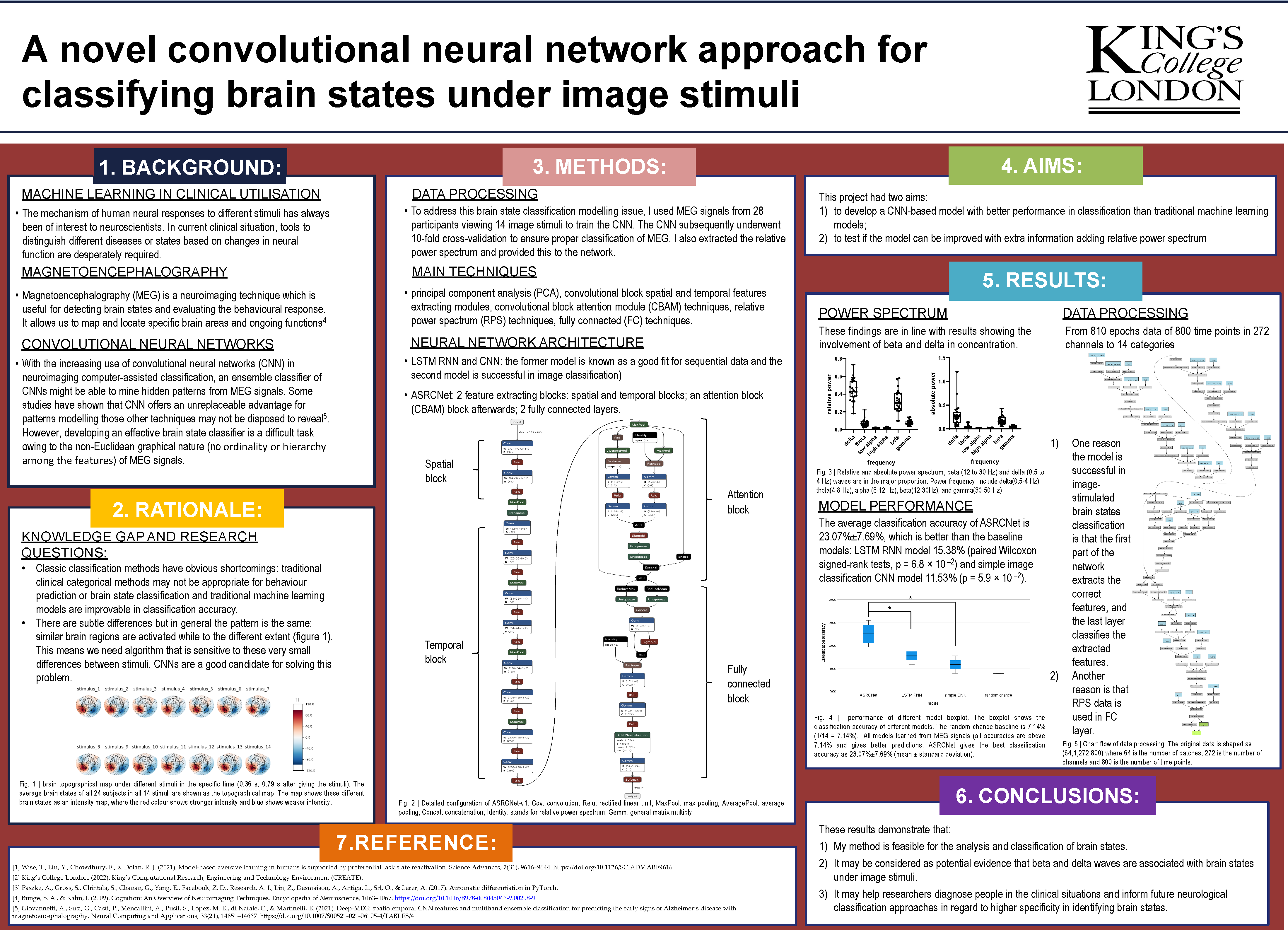
Background: The mechanism of human neural responses to different stimuli has always been of interest to neuroscientists. In the clinical situation, tools to distinguish different diseases or states are required. However, classic classification methods have obvious shortcomings: traditional clinical categorical methods may not be competent for behaviour prediction or brain state classification and traditional machine learning models are improvable in classification accuracy. With the increasing use of convolutional neural networks (CNN) in neuroimaging computer-assisted classification, an ensemble classifier of CNNs might be able to mine hidden patterns from MEG signals. However, developing an effective brain state classifier is a difficult task owing to the non-Euclidean graphical nature of magnetoencephalography (MEG) signals.

Objective: This project had two aims: 1) to develop a CNN-based model with better performance in classification than traditional machine learning models; 2) to test if the model can be improved with extra information adding relative power spectrum.

Methods: To address this brain state classification modelling issue, I used MEG signals from 28 participants viewing 14 image stimuli to train the CNN. The CNN subsequently underwent 10-fold cross-validation to ensure proper classification of MEG. I also extracted the relative power spectrum and provided this to the network. The following main techniques were applied in this research, principal component analysis (PCA), convolutional block spatial and temporal features extracting modules, convolutional block attention module (CBAM) techniques, relative power spectrum (RPS) techniques, fully connected (FC) techniques.

Results: In this research, my method was applied to the MEG dataset, the average classification accuracy is 23.07%±7.69%, which is much better than the baseline models: LSTM RNN model 15.38% (p = 6.8 × 10 ^–2^) and simple image classification CNN model 11.53% (p = 5.9 × 10 ^–2^). Relative power spectrum information (mainly beta and delta during this task) successfully informed the model improving its performance.

Conclusion: These results demonstrate that my method is feasible for the analysis and classification of brain states. It may help researchers diagnose people in the clinical situations and inform future neurological classification approaches in regard to higher specificity in identifying brain states.

Introduction

Machine learning in medical utilisation

Since Donald Hebb first composed the cell assembly theory stating the consistency between neuronal activity and cognitive processes (Brown & Milner, 2003; Shaw, 1986), the idea of neural networks started to stand out in public visibility. Until Frank Rosenblatt first developed and explored the basic ingredients of deep learning (DL) (Tappert, 2019), the only constraint that can slow our steps are applications of math methods. The last past decades have seen the quick and great revolution of artificial intelligence as the development of computer science. What the big breakthrough takes us close to the scientific field are the powerful tools that teach machines to learn about the physical world. Even though machine learning techniques have gradually built their presence in recent decades, the application in medical utilisation lags.

In the past centuries, neuroscientists have always been attempting to classify and predict the brain’s response to the visual world. Recently, with the rapid emergence of novel non-invasive techniques such as magnetoencephalography (MEG), electroencephalography (EEG) and magnetic resonance imaging (MRI), neuroscientists start to use these tools to solve the historical conundrum; and have made huge progress in the visual perceptual decoding or so-called “brain-reading” field (W. Huang et al., 2020). Each individual conscious experience is associated with a unique brain activity pattern so that it can be regarded as a fingerprint of specific brain activity. It is theoretically viable to read out one’s current idea with a specifically designed computer vision and neuroimaging pattern (Haynes, 2012). In this case, it might be possible that these “brain-reading” techniques can tell us that could be helpful with regard to clinical applications. Nowadays, many neural mechanisms have been elucidated. Although the current studies are mostly on a reflective proof of concept track (Hedderich & Eickhoff, 2021), it is promising that these approaches will pave the way and build a solid foundation in regard to clinical applications. In contrast to the classic understanding of some mental mechanisms, more and more researchers believe that traditional categories systems may twist the real cause of diseases or behaviours (Bzdok & Meyer-Lindenberg, 2018). To fill this gap, deep learning techniques have been introduced into disease diagnosis and classification. It can avoid being affected by people’s opinion bias but conversely get feedback from people so as to improve its learning ability from existing experience (Currie et al., 2019). Apart from disease classification, it is more profound to study human brain states under different conditions. Further studying of future state simulation has properly gained attention, especially on episodic future thought: the ability to rehearse events in mind, which may be going to happen in one’s life trajectory (Schacter et al., 2017; Szpunar, 2010).

Aversive state reactivation and replay

The aversive state is critical for harm avoidance, playing a vital role in wilderness survival and social life (Terranova et al., 2022). As part of the aversive state, the observational fear process promotes one’s capability of showing empathic fear when seeing other’s aversive situations. This process may benefit from the neural replay and reactivation of individuals. The process that current state simulation reinforces the existing memory network is called “reactivation” while the neural activity activation is named “neural replay”. The reactivation is based on past experience and in turn, promotes the storage of it, as well as facilitating the planning, inference and reward values updating (Wimmer & Shohamy, 2012; Wise et al., 2021). As mentioned in the previous section, one way to look at future thought simulation is to investigate memory reactivation.

Recent works have shown that neural replay and reactivation are prior important in avoidance behaviour (Wu et al., 2017), which may provide individuals with a prospective prediction based on the possible consequence simulation (Doll et al., 2015). Since then, it is known “which” correlates to the aversive state, the following step is figuring out to what extent neuronal activity is associated with behaviour. Naturally, it encourages researchers to try predicting one’s avoidance behaviour with the neuroimaging data recording. In recent years, more and more studies start to use neuroimaging classification to look for the inner mechanisms of brain states’ reactivation (Belal et al., 2018; Eichenlaub et al., 2020; Roscow et al., 2021). If we want to look at memory reactivation, what we need is really good decoding methods with neuroimaging data recordings. So, it’s important to optimise existing decoding methods as far as possible, which will set the scene for future related work.

Magnetoencephalography

Magnetoencephalography (MEG) is useful for detecting brain states and evaluating the behavioural response. It allows us to map and locate specific brain areas and ongoing functions (Bunge & Kahn, 2009). The principle of MEG is based on magnetic induction. It is widely known that when neurons are activated, electrical signals will be generated synchronously. According to the magnetic induction principle, when the electrical fields change, secondary magnetic fields are generated. The brain-evoked magnetic field strength is usually in the range of femto-tesla to pico-tesla, i.e., 10–15 to 10-12 tesla (Singh, 2014). With the precise MEG device and mathematical preprocessing methods, these tiny signals are able to be separated from the noise and collected. MEG records magnetic fields, from which can be inferred changes in the transmission of postsynaptic current between cortical neurons.

Compared to other neuroimaging methods, functional magnetic resonance imaging (fMRI) has high spatial resolution but a low temporal resolution (Dash, Sao, et al., 2019); electroencephalography (EEG) records the electrical field that may twist between skin and skull, and EEG is based to reference point location hence it is sensitive to small measurement error. Electrocorticography (ECoG) is an invasive method, so it is not suitable for healthy participants and some patients; MEG stands out for its higher spatial, temporal resolution and dynamic time sequentiality. At the same time, MEG, as a non-invasive method, has its specific advantage: low preparation time, which supports a possibility for most clinical conditions. Furthermore, as novel portable MEG devices come out, it creates opportunity for various ages participants and patients (Boto et al., 2018). MEG data records complex high-dimensional information about the brain network and the responding source locations, which is hard to collect with classic classification methods (Giovannetti et al., 2021). However, in the analysis period, it is a burden for researchers to do classification with MEG data: it is complex to correctly extract required signals during preprocessing, and lots of related experience is required when dealing with complex sensors and waveform patterns. Hence deep learning is expected to lighten the load of researchers, add the universal applicability of classification and increase the prediction accuracy. In this case, it is a challenge to choose the proper neural network.

Convolutional Neural Network

The CNN is a particular subtype of the neural network, which is effective in analysing images or other data containing high spatial information (Khan et al., 2018; Valueva et al., 2020) and also works well with temporal information (Bai et al., 2018). The same as the real neural networks in the brain, neurons in CNN process limited input data in a restricted receptive field and cooperate with each other by overlapping to cover the whole visual space (the filter extracting the features is called kernels). It is an automatic feature extraction process. Thus, it is now necessary to manually design feature extraction algorithms, which is required in traditional machine learning algorithms. It is also the main advantage of CNN to learn features from input data: avoiding the impact of artificial artefact in the algorithm design step. The main specialization of CNN is clearly the convolution part, which is a linear mathematic operation allowing extracting the nearby features of input data. The convolutional operation generates a series of machine-recognizable output features. It is suggested that the convolutional layer can be considered as a graphical pattern mining or feature extraction process (Li et al., 2018). What is more, previous research has shown the ability of CNN as a tool for analysing MEG data, which is in detail classifying brain activity and identifying potential neural sources (Zubarev et al., 2019). The process of generating the features map is following the sequential architecture, which is not like a cyclical recurrent neural network. A CNN model is usually composed of the input layer (the first layer where input data is passed in), multiple convolutional layers (feature extraction layers), alternative pooling layers (downsampling layer for feature maps), fully connecting layers (used to map the feature vectors obtained from previous feature extraction layers to the next layer), and output layers (the final layer where predictions are made). Inside each layer, activation functions are optional. A simple CNN network is shown as an example in figure 1. The convolutional layer receives input data, apply the convolution process to the data, and passes data to the following step. In the convolution function shown in equation 1, the f stands for input data; k stands for kernel filter, m, n respectively stands for the result matrix rows and columns index:

$$\begin{matrix}
G\lbrack m,\ n\rbrack = \ (f*k)\lbrack m,\ n\rbrack = \ \sum_{i = 1}^{m}\ \sum_{j = 1}^{n}\ \ k\lbrack i,\ j\rbrack f\lbrack m - i,\ n - j\rbrack\ \ (1) \
\end{matrix}$$

As shown in figure 2 (A), a kernel filter is applied to the input data pixel: after summing up input values and filter, a result value is generated and passed to the next step. With all similar processes conducted step by step, a feature map is generated. Afterwards, the max pooling step (figure 2 (B)) comes to decrease the dimensions of data in order to keep more neurons activated which is reported to reduce the overfitting as well (Y. Huang et al., 2015).

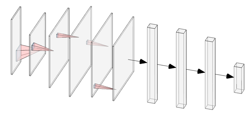
Figure 1. A simple CNN architecture illustration (5 convolutional layers and pooling layers, 3 fully connected layers)

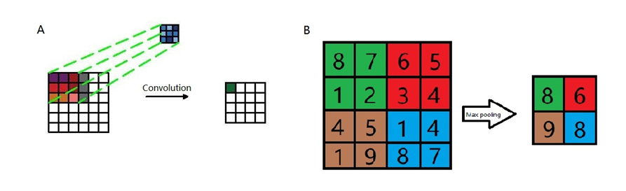
Figure 2. Convolution illustration (A), a 3*3 kernel filter (blue) is applied to a 6*6 input data (red) and give an output (green) as 4*4 (feature map). Max pooling illustration (B), data transformation is processed from 4*4 input to 2*2 output.

In previous research, sequence data were usually analysed with the recurrent neural network (RNN) while the convolutional neural network (CNN) was used for image prediction. However, recent works have demonstrated the effectiveness of CNN in time-sequential data (Bai et al., 2018) where CNN even have a longer effective memory. It provides us with the theoretical basis for utilizing various CNN models in behaviour prediction. CNN has also been used for MEG classification in recent years: previous research has successfully predicted different diseases such as brain tumours (Rajasree et al., 2021) and Alzheimer’s disease (Aoe et al., 2019; Giovannetti et al., 2021). In fact, some studies have shown that CNN offers an unreplaceable advantage for patterns modelling those other techniques may not be disposed to reveal (Giovannetti et al., 2021). However, it is still an emergent topic to use deep learning instead of the classic machine learning method. As a special machine learning technique, deep learning benefits from the fast development of high-performance computation (HPC). One example is that deep learning can use the CUDA framework to accelerate training. As the GPU accelerators become more and more performance and energy-consuming effective (Faraji et al., 2016), the cheaper computation source becomes more and more available. Some evidence has shown that deep learning performs better than the classic machine learning methods when doing MEG classification (Aoe et al., 2019; RaviPrakash et al., 2020; Zheng et al., 2020). In addition to these the ability to recognize temporal and spatial data patterns, CNN has the unique character of sharing weight among neurons in a convolutional layer (Anelli et al., 2021). In this case, the parameters quantity reduces sharply which benefits analysing complex structured MEG data.

Band power and Transfer learning

CNNs are expected to have good performance for extracting features from MEG data, but the performance can be boosted by augmenting the data we feed into them. Here are some ways I did this with MEG data. MEG signals reflect brain activity, in which the brainwave can be deposed into different frequency power bands, such as delta (0.5-4 Hz), theta (4-8 Hz), alpha (8-12 Hz), beta (12-30Hz), and gamma (above 30 Hz). And these different brainwave frequency bands usually are associated with different brain states, such as the alpha band has been implicated in visual attention (Rohenkohl & Nobre, 2011). and the beta band is usually associated with anxiety (Einöther et al., 2013). That is why I think particular frequency bands might be important in helping classify accurately. In order to understand if it is available to extract critical information from the aversive state, it may be viable to extract different power bands and analyse them as a neural activity representation. One drawback of this method is it may reduce the available temporal information in MEG data, but it can not be denied that it provides an excellent and reliable method to study brain states (Newson & Thiagarajan, 2019).

However, the trained model may not be suitable for data collected under other conditions. Between the MEG device and its recording source location, there are the skull, skin and even air, which may all affect the signals we get: the deeper source is, the more affected it will be. In addition to these confounds, the geometric shape of the skull which varies a lot between different people, also affects a lot (Hagemann et al., 2008). In order to generalize the model, power spectrum standardization and relative power computation are necessary. Moreover, it is reported that transfer learning can help to improve learning efficiency by reusing or transferring learnt parameters (Karimpanal & Bouffanais, 2018). In this case, transfer learning may reduce the influence of these confound factors and increase the generality of models.

Transfer learning is the machine learning technique which allows a network to learn in one condition and improve its performance under another relevant condition. It is an optimization method to inform new task learning with relative learnt knowledge (Soria Olivas & IGI Global., 2010). For the transfer learning process, only part of the model parameters is trained and adjusted, which is called “tuning”. If all network parameters are opened for training, it is easy to fall into the state of overfitting the target training set, thereby reducing the generalization performance of the model. The first few layers of the network are generally used for feature extraction. If the difference between the source task and the target task is not quite significant and the model has achieved good performance in the source task, there is no need to perform training from the beginning (Karimpanal & Bouffanais, 2018). In this case, the transfer learning technique solves the small data availability problem: with a small amount of data, it helps eliminate the overfitting problem and reduce the model training time. Some evidence suggests that it can keep at a high accuracy level and saves 90% time (Dash, Ferrari, et al., 2019). It has been widely used to transfer the weight or bias of the current network to a newly trained network with the object of faster convergence and better performance.

For aversive state reactivation prediction, previous studies have provided an approach with logistic regression methods and get a good accuracy (Wise et al., 2021) With a different approach (CNN) we could probably detect brain state reactivation with much better accuracy and learn a lot more about it. My first aim is to optimize the model with new techniques such as CNN and apply spectrum power. The second aim is to generalize the model by informing one participant model with other participants’ data. I assume that: first, the performance of the CNN model is better than traditional machine learning models; second, adding the power spectrum to augment data will improve the performance as well.

Materials and Methods

Dataset

The participants, study design, data collection and preprocessing sections and relevant information are included and published in the paper "Model-based aversive learning in humans is supported by preferential task state reactivation" (Wise et al., 2021). Open access to the original MEG data can be found in the public repository: https://openneuro.org/datasets/ds003682. In total 28 participants took the task. The task is designed as follows: participants were required to sit with the MEG device in front of a monitor, where 14 images were shown. The recording duration of each stimulus is 1.29 seconds (from 0.5 before to 0.79 after image is shown). MEG data were collected with CTF 275-channel axial gradiometer system (CTF Omega, VSM MedTech). In the preprocessing session, the Maxwell filter was applied to remove noise firstly. Then a high pass filter above 0.5 Hz and a low pass filter below 45 Hz were applied. Afterwards, signal components were separated with independent component analysis (ICA) to isolate noise-related components in the setting of finding components which explain 95% variance. To reduce information loss, MEG data was upsampled and the window width of data was set as 800 time points (Aoe et al., 2019) when training the model to get better performance.

Power spectrum extraction

In order to compute the relative power (percentage power) of MEG signals, the first step is to extract the power band with the specific frequency. The frequency bands were chosen to be delta (0.5-4 Hz), theta (4-8 Hz), low alpha (8-10 Hz), high alpha (8-12 Hz) beta (12-30 Hz), and gamma (above 30 Hz). Actually, the gamma frequency was below 50 Hz because it is impossible to detect any information above 50 Hz as the data are sampled at 100 Hz.

Firstly the power spectral densities (PSD) and frequency of each band were derived using Welch’s method with mne.time_frequency.psd_array_welch() function provided by MNE-Python (Percival & Walden, 1993; Slepian, 1978). The reason for choosing this function is this function gives a single value for each trial but other methods that give you power at each timepoint. Then the PSD of each band was integrated with the frequency as spacing point using composite Simpson’s rule. The absolute power in a specific location is the average number of the power from several adjacent electrodes. The relative power is the ratio of the absolute power of a band to the total band power in all frequencies. As shown in equation 2, the r represents the relative power of a frequency band, the a stands for absolute power of the same frequency band, Pi ‘s are the absolute power in all frequency bands:

$$\begin{matrix}
r = \frac{a}{P_{t}} = \ \frac{a}{\sum_{\ }^{\ }{P_{i}\ }}\ \ (2) \
\end{matrix}$$

Eventually, the absolute and relative power bands are transformed from input data in $\mathbb{R}$C×T (where $\mathbb{R}$ is a vector space) to $\mathbb{R}$C×F, where C is the number of channels, T is time points and F is the number of frequency bands, i.e., 6 here.

Neural Network architecture

In order to classify different 14 categories brain states under 14 stimuli based on MEG signals, I proposed a CNN model ASRCNet-v1. The input data are MEG recordings from 24 subjects (4 were removed because of its information missing). In order to augment the data, the input of last fully connected layer was concatenated with relative power bands in all frequencies. The neural network structure of ASRCNet-v1 was developed based on the previously reported model EnvNet-v2 and MNet (Aoe et al., 2019; Tokozume et al., 2017; Tokozume & Harada, 2017), which was used to classify environmental sounds and Alzheimer’s diseases. The detailed configuration of ASRNet-v1 is as demonstrated in figure 3 and the data processing is demonstrated in figure 4. There are three convolutional blocks in total: two feature extracting blocks: spatial and temporal blocks; and a CBAM block after them. In the first convolutional layer, the global features were extracted with a large filter, which has the same kernel width as the channel number of inputs. The kernel length of the first layer is set to be 64. The first layer generates a feature map in $\mathbb{R}$S×1×T’ from input data in $\mathbb{R}$C×T, where the T is larger than T’s. The C (number of channels) is larger than S (number of spatial filters) such that the channel dimension is reduced. The second convolutional layer in the spatial block generates a feature map in $\mathbb{R}$S’×1×T’’ with frequency features then. Afterwards, the data is downsampled with a max pooling layer and swapped along the axis between S and 1, i.e., from $\mathbb{R}$S’×1×T’’ to $\mathbb{R}$<!-- -->{=html}1×S’×T’’. This operation allows data being considered as the image changing the convolutional direction (Tokozume et al., 2017). The second block consists of eight convolutional layers and four max pooling layers. The kernel size of convolutional layers is small and decreases every two layers in order to extract local frequency temporal features from the output feature map from the previous layer. Relu is the activation function for all convolutional layers in the spatial block. Max pooling layers are attached after every two convolutional layers.

The attention block is composed of 2 parts: the channel attention module and the spatial attention module. Two modules help model focus more on the important information: channel dimension and spatial dimension. First, for the channel attention module, input data process average pooling and max pooling separately, where the average pooling layer is used to aggregate spatial information and the max pooling layer is used to maintain more extensive and precise context information as images’ edges. The outputs are passed to an MLP (multilayer perceptron) network with the same weight. The MLP layer has a bottleneck. The width and length or the number of neurons in this MLP layer are decided by a reduction ratio of 16. Then the sum of two outputs from the MLP layer is given to the sigmoid activation function in order to project values in features map into $\mathbb{R \in}(0,1)$. Finally, the channel attention module returns a feature map as the product of input and calculated scale. Compared with the channel attention module, spatial attention seems to be simpler, which includes one convolutional layer and the sigmoid activation function. The same as the channel attention module, the spatial attention module returns a feature map as the product of input from the previous module and calculated scale in this module.

Then the first fully connected layer (FC) comes to play the role of classifier, which is projecting the “distributed feature representation” of the feature map to sample labels space $\mathbb{R}$L, where L is the number of features. In the object of data augmentation, the input is concatenated with relative power bands in all frequencies. The following step is another FC layer, which finally generates 14 features corresponding to the number of categories. At last, data is passed to the softmax activation function to convert the numbers vector into the probabilities vector. To avoid overfitting, 30 % dropout is applied after the last 4 spatial convolutional layers and 50 % dropout is applied after the first fully connected layer (Srivastava et al., 2014); batch normalization is applied to boost the speed of learning (Ioffe & Szegedy, 2015).

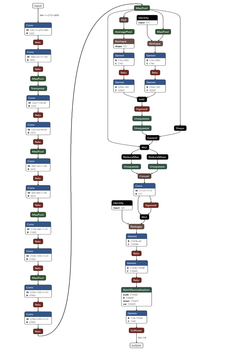
Figure 3. Detailed configuration of ASRCNet-v1. Cov: convolution; Relu: rectified linear unit; MaxPool: max pooling; AveragePool: average pooling; Concat: concatenation; Identity: stands for relative power spectrum; Gemm: general matrix multiply

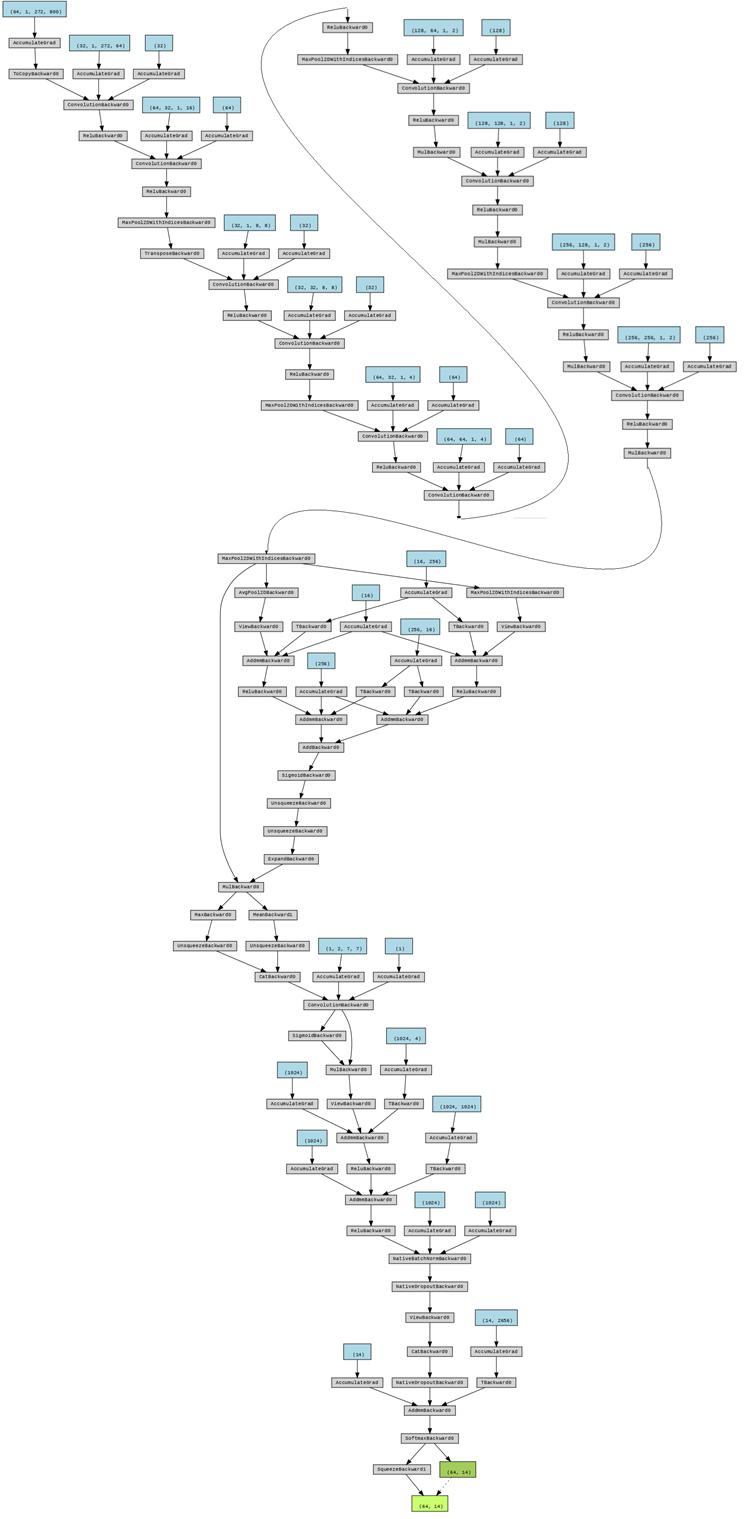
Figure 4. Chart flow of data processing. The original data is shaped as (64,1,272,800) where 64 is the number of batches, 272 is the number of channels and 800 is the number of time points.

Model training and testing

The input data is a total of 900 epochs of 800-time-point MEG signals from 272 channels. At the beginning, the data was separately processed directly with the neural network and the Fourier transformation. The latter process provides neural network with relative band power in frequency delta (0.5-4 Hz), theta (4-8 Hz), alpha (8-12 Hz), beta (12-30Hz), and gamma (above 30 Hz). The input data is shuffled and scaled with variance scaling method, which reasonably preserves the dynamic range of data, before being fed into the model. The first step is to normalize all input data for the reason that normalization step can generalize the statistical distribution of uniform samples, which is expected to enhance the training performance. The normalization process is as shown in equation 3, where m is the total number of data and x represents data, makes the average value and standard deviation of data in each channel to be located in the range between 0 and 1:

$$\begin{matrix}
{x_{i}}^{‘} = \frac{\left| x_{i} - \frac{1}{m}\sum_{1}^{m}\ x \right|}{\sqrt{\sum_{1}^{m}\ x^{2}}}\ \ (3) \
\end{matrix}$$

In every training period, the input is one piece of a small segment of 64 batches of MEG signals segmented with non-overlapped 800-time-point time windows. The cross-entropy loss function was chosen to train the model because of its better performance in computing losses for discrete distributions. I chose SGD to be the optimizer because it is reported to have a better generalization capacity compared with Adam even though it may converge slower (Hardt et al., 2015). For the SGD optimizer, I set the initial learning rate as 0.0005, and momentum to 0.9. Specifically for the parameters in the second FF layer, a weight decay as 0.0005 is set keeping away from overfitting. The initial weight is randomized, which is because it is reported there is no obvious performance promotion with manually weight initialization (Hoshen et al., 2015). In order to improve training efficiency and avoid overfitting, I adapted the update step: I used the dynamic learning rate when the valid loss approaches a plateau (function 4, where $\lambda$ represents learning decay and L represents valid loss). The patience of the dynamic learning rate is set to 1, the threshold is set to 0.001 and learning rate decay is set to 1e-8. Since there are a large number of features during training, in order to avert overfitting, I introduced L2 regularization (ridge regularization) with the regularization parameter lambda to 0.001. After the trial with model performance in different checkpoints, early stopping was finally adopted when the number of epochs reaches around 130 in case of overfitting.

$$\begin{matrix}
\alpha_{t + 1}\ = \ \left{ \begin{matrix}
\alpha_{t} \times \lambda & if\ L_{t + 1} > \ \ L_{t} \
\alpha_{t} & if\ L_{t + 1} \leq \ \ L_{t} \
\end{matrix} \right.\ \ \ (4) \
\end{matrix}$$

Finally, the possibility of each label is generated in the model. It eventually gives only one “most possible” label after comparing the possibility in all labels. In order to prove the validity of this CNN model. ASRCNet-v1’s performance is evaluated with 10-fold cross-validation, where 1 in 10 sets is used as validating set every time.

Result

The key results of the article are summarised and given in this section. This section first offers auxiliary findings with the whole dataset and furthermore demonstrates results using a single MEG dataset (i.e., a single subject). The accuracy measure is utilized to compare the performance of various models. All models had previously undergone testing on participant 1 to provide an initial indication of performance. The suggested model solution is validated across all of the participants once all models have been evaluated on participant 1. Additional tests are specifically run on the best model ASRCNet and other two main baseline models (LSTM RNN and simple CNN). For models tested on all subjects, model training was done within each participant, trained and evaluated only using its individual recording MEG data. Additionally, I set the windows of input data to 800 ms enabling an accurate comparison of several test models. Relative power spectrum is introduced to the training improving performance of models. Moreover, average topographical maps are graphed as the representation of the MEG signals intensities in the anatomical brain, illustrating the general topographic maps of brain states from different stimuli in brain states reactivation tasks.

Topographical map

The global anatomical brain maps are generated with concatenated dataset and were back fitted to MEG recordings. The average MEG signals with different stimuli are calculated and graphed showing commons and differences among various brain states under different stimuli. In the brain states reactivation process, under the different stimuli, the topographical maps all look very similar. There are subtle differences but in general the pattern is the same: similar brain regions are activated while to the different extent (figure 5). This means we need some kind of algorithm that is sensitive to these very small differences between stimuli.

The result shows the rationality of extracting features of brain states under different stimuli. It may suggest that stimulus representations are in the downstream temporal region or visual cortex. Thus, as the following training results showed, ASRCNet is an effective and reasonable approach to classifying these states.

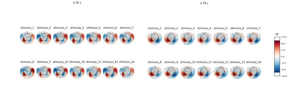
Figure 5. brain topographical map under different stimuli in the specific time (0.36 s, 0.79 s after giving the stimuli). The average brain states of all 24 subjects in all 14 stimuli are shown as the topographical map. The map shows these different brain states as an intensity map, where the red colour shows stronger intensity and blue shows weaker intensity. The brain areas that are activated are concentrated in the downstream temporal region or visual cortex.

Power spectrum

In order to determine the effect of different brain wave frequencies, power spectral density (PSD) at all 272 channels is calculated. The 6 power bands are divided by the sum generating 1632 decoding features (272 channels for each of the 6 frequency bands). I analysed the power spectrum in all frequencies of input 800-time-point MEG signals for different participants. The results show that beta and delta waves are in the large and major proportion (figure 6). It may be considered as potential evidence that beta and delta waves are associated with not only anxious thinking, and active concentration (Baumeister et al., 2013), but also the aversive state. In the following classifier task, these findings are in line with results showing the involvement of beta and delta in concentration.

Figure 6. Relative and absolute power spectrum (average of 24 subjects), beta (12 to 30 Hz) and delta (0.5 to 4 Hz) waves are in the major proportion

Classification of multiple brain states reactivations

In order to classify the brain states reactivation with different given image stimuli (figure 7), ASRCNet-v1, the classifier is developed. It is trained with MEG signals for each of the images. The representative MEG signals for each reactivation states that ASRCNet-v1 accurately identified is displayed in figure 8. A sample of an 800-time-point segment of the preprocessed MEG signals is displayed in the panel, where each contains 900 epochs. In these samples, there are no spikes or other distinctive abnormal waveforms. For every single training dataset from various participants, 900 of in total 900 events passed the rejection process. Therefore, none of these signals are removed because of bad channels. It is because the rejection algorithm was purposefully designed to be inclusive. All data were deliberately included because the CNN model should be robust to noise in the data. It is suggested that ASRCNet-v1 correctly categorised the MEG signals during aversive state by utilising features that not presents in the typical classification.

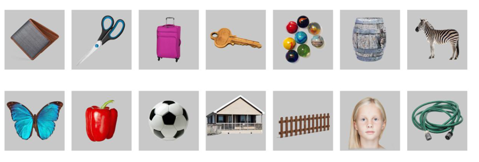
Figure 7. image stimuli in different brain states reactivation tasks (Wise et al., 2021), from left to right, above to bottom are labelled as stimulus_i.

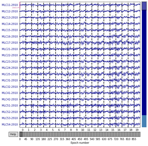
Figure 8. representative MEG signal which is classified by the ASRCNet-v1 (from one sample participant)

Principal component analysis (PCA) (30 to 50 out of 272 channels) was tested to be applied to the input data before feeding data into the model. But the result shows that PCA does not obviously improve the classification performance of ASRCNet-v1. The classification accuracy was not obviously affected when PCA was applied. In the beginning, I didn't get satisfactory learning convergence results. When the input data values are clipped to be in of standardized bounds, the learning curves became smooth and the valid loss gradually decreased step by step.

Since there are 14 stimuli and the chances for all stimuli are equal, the random prediction accuracy is expected to be 7.14% (1/14 = 7.14%). The classification accuracy of ASRCNet-v1 is around 23.07%, which is clearly higher than random chance. LSTM RNN gives an accuracy of about 15.38% while simple CNN only gives a mean accuracy of 11.53%. I compared the performance of different models (figure 9) and found it is suggested that ASRCNet-v1 outperformed any other simple approach (LSTM RNN, simple CNN with 2 convolutional layers and 1 pooling layer). Compared with the other classification approach, ASRCNet-v1 exhibits the best classification performance (p = 6.8 × 10 –2 for LSTM RNN, p = 5.9 × 10 –2 for CNN, paired Wilcoxon signed-rank tests). The best classification accuracy of ASRCNet-v1 is able to reach 33.33%. The classification accuracy variety between simple CNN and ASRCNet may suggest that the classification depends on some event-independent signal: the temporal and spatial features. To which extent the performance is a result of the detected differences in the temporal and spatial features of MEG signals, remained to be explored.

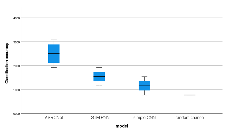
Figure 9. performance of different model boxplot. The boxplot shows the classification accuracy of different models. The random chance baseline is 7.14% (1/14 = 7.14%). All models learned from MEG signals (all accuracies are above 7.14% and gives better predictions. ASRCNet gives the best classification accuracy as 23.07%±7.69% (mean ± standard deviation).

Discussion

In this section, I am going to discuss the experimental results, findings, and potential future work. The focus of this paper is to explore the potential of deep learning, especially CNN to classify the aversive brain states associated with visual images. The MEG signals are complex and have low signal-to-noise ratios data structures. What is more, the aversive brain states parameters are continuous variables. Therefore, the aim is to solve a complex classification task. To optimally address this problem, a CNN model ASRCNet (inspired by Mnet and EnvNet, which was used in MEG data) is proposed as the deep learning solution in this research because of its ability to extract complex patterns from raw input data. One focus is to understand whether the CNN model is able to perform the decoding task. The analysis has been evaluated in two distinct steps: First, two well-known architectures (LSTM RNN and CNN: the former model is known as a good fit for sequential data and the second model is usually used in image classification) were selected as baseline models for the purpose of understanding the potential of general-purpose DL models that are not specific to MEG analysis. Second, I test the prediction and classification ability of the CNN-based architecture specially designed for MEG recordings. The results show that ASRCNet provide better performance compared to the other two baseline models. Since the model is specifically designed to extract features from MEG recordings, it can be considered an option in the field of brain state classification.

I trained a novel deep neural network ASRCNet to classify 14 brain states using data from MEG recordings. It can distinguish brain states under different image stimuli with an accuracy at least as good as, or even higher than the baseline pipeline. ASRCNet allows the extraction of spatial and temporal information from the informative MEG data. It is suggested that classification decisions are unlikely to be associated with activities that are unrelated to the task itself, for example, mind wandering. The trained ASRCNet successfully classifies brain states with relatively high accuracy and specificity. Previous research has been focusing on common symptoms of psychopathology, but less on the domain of aversive states. This is a study using MEG signals to classify different aversive brain states with a classifier. The high specificity for all states suggests that ASRCNet will help improve our understanding of the human cognitive image process. One thing we can do with such a CNN classifier is to look at state reactivation in cognitive tasks. Moreover, this classifier is expected to be applied in clinical studies in order to diagnose nonorganic neurological diseases. As shown in the topological map in the result section, these brain states are hard to classify with the naked eyes. The information from such computer-aided diagnosis may be a novel biomarker for these diseases in clinical practice.

The advantage of using this neural network is its comprehensive training process, entirely based on gradient descent-based optimization without intermediate steps. As research develops toward explainable artificial intelligence (XAI), the parameters of a model may be going to have a direct and explainable connection to their task. On the separate brain states classification task, ASRCNet also performs on par with state-of-the-art, potentially making it a general method for other neuroimaging data. What is more, as shown in the result section, the classification accuracy varies a lot between simple image classification CNN and ASRCNet. One reason the model is successful in classification is that the first part of the network learns to extract the correct features, while the last layer classifies the extracted features. It may suggest that the classification of such brain states depends on some event-independent temporal and spatial features signal. Some evidence suggests that using features automatically extracted with deep learning models rather than manually selected, is able to help achieve the highest levels of accuracy compared to other machine learning approaches. It is reported that most of the best ImageNet is achieved by using some kind of data augmentation, instead of feature engineering and dimensionality reduction (de Bardeci et al., 2021). However, it was reported that logistic regression may achieve better classification accuracy than ASRCNet (Wise et al., 2021). It may be because of the algorithmic Incompleteness of the current model. Future work on improving the algorithm may improve the performance of CNN models.

ASRCNet is a relatively robust approach among different subjects. In this research, 14 different stimuli were applied to 24 subjects (data from 4 subjects were removed because of the smaller segment length). ASRCNet successfully classifies states in 24 different subjects with high accuracy, demonstrating the robustness of the CNN model. However, the data itself used in the research has potential for improvement: the 13th stimulus is a face picture, which may be different from other stimuli reflecting brain states (Rapcsak, 2019). What is more, it is concerned that the trained model may have difficulty classifying brain states using data recorded by another MEG scanner. Improvements in current source estimation and alignment techniques may make the method adaptable to different MEG scanners (Pettersen et al., 2006). Apart from the robustness, the size of the data itself may also affect the classification accuracy. A limitation of this experiment is, the same as in most other studies, the cross-validation approach was performed during the validation process, rather than using a separate test dataset. It was reported that using a separate test set in the DL model may help yield the highest level of validity in the results (de Bardeci et al., 2021). Although superficially, it is a relatively advanced practice to use data from the same subject in the training and test sets, there is room for improvement. A possible improvement is to create additional test sets beyond the limited availability of data. Due to the high inter-individual specificity and intra-individual stability of MEG data, it is difficult for the network to learn common features between subjects. The current approach of the model is to recognize different subjects by identifying individual MEG features of different subjects. Therefore, even though the network can achieve high levels of accuracy, classification and prediction will be unpredictable when it is applied to entirely new datasets from different subjects. The application of transfer learning methods with the small tuning of part of model parameters may be a possible solution. However, when performing transfer learning, it is generally assumed that different tasks are related. In this case, how to define the correlation and mathematically describe the strength of the correlation between tasks are subjective decisions that are biased toward researchers. The image classification-related studies usually use ImageNet as a pre-trained model for transfer learning because the large dataset of ImageNet itself ensures that the trained model has high generalization. But when we use a small dataset such as in this experiment, transfer learning may not only fail to achieve the expected result but result in negative transferring which is even worse than training a network from nowhere. For example, AlphaGo Zero learned from zero without any supervision or using chess manual data but achieves higher performance than AlphaGo Lee which is based on chess manual replays (Silver et al., 2017). Therefore, how to perform correct and effective transfer learning is one of the focuses of future work.

Deep learning from scratch is often difficult with limited amounts of data. However, even with the limited amount of data in this study, I successfully classified 14 types of brain states. One reason for this success is that I enlarged the dataset by dividing each subject's 1170 seconds of data into 900 segments of 1.3-second time data, allowing me to train 14 classes using approximately 25200 segments. The data amount is slightly less than the amount of MNIST, a database of handwritten digits that is often used to train deep neural networks, but still shows that I have a reasonable amount of data to train a network of such size (Yann LeCun et al., 2012). However, during the training process, the training data generally has a tendency to overfit even though I applied dropout (randomly ignored neurons in network) and batch normalization (normalizes input mini-batches from last layer). The proposed CNN model ASRCNet may benefit from the increase in dataset size. It improves with more training data because deep learning performance is reported to improve significantly with larger datasets (Greenspan et al., 2016). Therefore, it can be taken into account to train this model with more data in hopes of improving model performance. In addition, more research has shown that MEG and EEG provide complementary information, and other modalities such as MRI also provide additional useful information. Using data from multiple method sources at the same time may improve model performance (Dale & Sereno, 1993; Sharon et al., 2007). In future work, combining MEG signal data with EEG to create a multimodal data input may help improve the accuracy of brain states classification.

In this ASRCNet, the integration of the relative power spectrum improves the CNN model’s performance. Since the beta and delta waves mainly encode perceptual information, the relative power spectrum ensemble adds relevant information to the model so that the different band power values can inform the network. Therefore, the model can adjust the weights accordingly. Additionally, the relative power spectrum may also add valuable information about artefacts or ambient noise (Anelli et al., 2021). All these deep learning models overfit the training dataset more or less, even applied regularization techniques like dropout and batch normalization. The additional information provided by the relative power spectrum ensemble helps the model to generalize. There is still room to improve the model’s performance as the aspect of power spectrum extraction. In the process of relative power spectrum extraction, the wavelet transform can be considered as an optional alternative to Fourier analysis for the reason that the wavelet transform has the multi-scale analysis ability to extract features from the dataset and generate input images for training the model. Compared with the Fourier transform, the wavelet transform is a local transform of temporal and frequency data, so it can more effectively extract information from the signal by performing multi-scale refinement analysis with operations like scaling and translation (Yu & Guowen, 1994), thus has the potential to solve some difficult problems that Fourier transform cannot deal with. Fourier transform can only get a frequency spectrum, but wavelet transform can get a temporal frequency spectrum which not only the frequency can be obtained, but also the time can be located. Some recent studies successfully use the wavelet packet decomposition method to extract time-frequency features and use a dynamic frequency feature selection algorithm to select the most accurate features for each subject (Luo et al., 2016). However, other studies have shown the drawback of wavelet packet decomposition: although this method improves the classification accuracy, it requires a lot of work to select the most suitable features for each subject, and the feature extraction for different target individuals is poorly general (Dai et al., 2020). Only considering the power spectrum is quite limiting at the current moment. The convolutional operation executed by most popular machine learning libraries in deep learning is actually computing the correlation measurement (Graves, 2012). Future work investigating state classification and reactivation should also take steps to measure event-related desynchronization and synchronization in the context of the data generated.

Another idea to optimize the model is to replace the fully connected layer with global average pooling. The model holds a redundancy of fully connected layer parameters where fully connected layer parameters can account for about 80% of the entire network parameters. Some recent network models with excellent performance, such as ResNet, are trying to use global average pooling (GAP) layer instead of a fully connected layer for fusion. For the learned deep features, loss functions such as SoftMax are still used as the network objective function to guide the learning process (Liu & Zeng, 2022) Some evidence suggests that networks that replace a fully connected layer with a GAP layer may have better classification performance (Wei et al., 2018). However, other studies have pointed out that when applying transfer learning, the fine-tuned results of networks without fully connected layers are worse than those with fully connected layers. Therefore, fully connected can be regarded as a guard for model representation capabilities, especially in the case that there are big differences between the source domain and the target domain, the redundant parameters of FC can maintain a fine model capacity to ensure the migration of model representation capabilities (Zhang et al., 2018). Future work can explore the role of the GAP layer and fully connected layer in detail.

ASRCNet can extract and analyze features that deep learning neural networks use for classification, which may help researchers understand brain states better. The inherent hidden patterns in brain states and related brain neural activity that deep learning may reveal some fundamental mechanisms behind human behaviour. To the extent these can be explained, researchers are encouraged to apply these sophisticated deep learning modelling techniques to obtain accurate classification and prediction results and to generalize the results more carefully in a wider range of conditions. Moreover, understanding the relevant studies that extract these hidden patterns can increase and deepen our understanding of the brain state electrophysiological characterization.

Reference

Anelli, M., Lauri, S. P., Advisor, P., & Zubarev, M. I. (2021). Using deep learning to predict continuous hand kinematics from magnetoencephalographic (MEG) measurements of electromagnetic brain activity. www.aalto.fi

Aoe, J., Fukuma, R., Yanagisawa, T., Harada, T., Tanaka, M., Kobayashi, M., Inoue, Y., Yamamoto, S., Ohnishi, Y., & Kishima, H. (2019). Automatic diagnosis of neurological diseases using MEG signals with a deep neural network. Scientific Reports, 9(1). https://doi.org/10.1038/S41598-019-41500-X

Bai, S., Kolter, J. Z., & Koltun, V. (2018). An Empirical Evaluation of Generic Convolutional and Recurrent Networks for Sequence Modeling. https://doi.org/10.48550/arxiv.1803.01271

Baumeister, J., Barthel, T., Geiss, K. R., & Weiss, M. (2013). Influence of phosphatidylserine on cognitive performance and cortical activity after induced stress. Http://Dx.Doi.Org/10.1179/147683008X301478, 11(3), 103–110. https://doi.org/10.1179/147683008X301478

Belal, S., Cousins, J., El-Deredy, W., Parkes, L., Schneider, J., Tsujimura, H., Zoumpoulaki, A., Perapoch, M., Santamaria, L., & Lewis, P. (2018). Identification of memory reactivation during sleep by EEG classification. NeuroImage, 176, 203–214. https://doi.org/10.1016/J.NEUROIMAGE.2018.04.029

Boto, E., Holmes, N., Leggett, J., Roberts, G., Shah, V., Meyer, S. S., Muñoz, L. D., Mullinger, K. J., Tierney, T. M., Bestmann, S., Barnes, G. R., Bowtell, R., & Brookes, M. J. (2018). Moving magnetoencephalography towards real-world applications with a wearable system. Nature 2018 555:7698, 555(7698), 657–661. https://doi.org/10.1038/nature26147

Brown, R. E., & Milner, P. M. (2003). The legacy of Donald O. Hebb: More than the Hebb Synapse. Nature Reviews Neuroscience, 4(12), 1013–1019. https://doi.org/10.1038/NRN1257

Bunge, S. A., & Kahn, I. (2009). Cognition: An Overview of Neuroimaging Techniques. Encyclopedia of Neuroscience, 1063–1067. https://doi.org/10.1016/B978-008045046-9.00298-9

Bzdok, D., & Meyer-Lindenberg, A. (2018). Machine Learning for Precision Psychiatry: Opportunities and Challenges. Biological Psychiatry. Cognitive Neuroscience and Neuroimaging, 3(3), 223–230. https://doi.org/10.1016/J.BPSC.2017.11.007

Currie, G., Hawk, K. E., Rohren, E., Vial, A., & Klein, R. (2019). Machine Learning and Deep Learning in Medical Imaging: Intelligent Imaging. Journal of Medical Imaging and Radiation Sciences, 50(4), 477–487. https://doi.org/10.1016/j.jmir.2019.09.005

Dai, G., Zhou, J., Huang, J., & Wang, N. (2020). HS-CNN: a CNN with hybrid convolution scale for EEG motor imagery classification. Journal of Neural Engineering, 17(1), 016025. https://doi.org/10.1088/1741-2552/AB405F

Dale, A. M., & Sereno, M. I. (1993). Improved Localizadon of Cortical Activity by Combining EEG and MEG with MRI Cortical Surface Reconstruction: A Linear Approach. Journal of Cognitive Neuroscience, 5(2), 162–176. https://doi.org/10.1162/JOCN.1993.5.2.162

Dash, D., Ferrari, P., Heitzman, D., & Wang, J. (2019). Decoding Speech from Single Trial MEG Signals Using Convolutional Neural Networks and Transfer Learning. Proceedings of the Annual International Conference of the IEEE Engineering in Medicine and Biology Society, EMBS, 5531–5535. https://doi.org/10.1109/EMBC.2019.8857874

Dash, D., Sao, A. K., Wang, J., & Biswal, B. (2019). How many fmri scans are necessary and sufficient for resting brain connectivity analysis? 2018 IEEE Global Conference on Signal and Information Processing, GlobalSIP 2018 - Proceedings, 494–498. https://doi.org/10.1109/GLOBALSIP.2018.8646415

de Bardeci, M., Ip, C. T., & Olbrich, S. (2021). Deep learning applied to electroencephalogram data in mental disorders: A systematic review. Biological Psychology, 162, 108117. https://doi.org/10.1016/J.BIOPSYCHO.2021.108117

Doll, B. B., Duncan, K. D., Simon, D. A., Shohamy, D., & Daw, N. D. (2015). Model-based choices involve prospective neural activity. Nature Neuroscience, 18(5), 767. https://doi.org/10.1038/NN.3981

Eichenlaub, J. B., Biswal, S., Peled, N., Rivilis, N., Golby, A. J., Lee, J. W., Westover, M. B., Halgren, E., & Cash, S. S. (2020). Reactivation of Motor-Related Gamma Activity in Human NREM Sleep. Frontiers in Neuroscience, 14. https://doi.org/10.3389/FNINS.2020.00449

Einöther, S. J. L., Giesbrecht, T., Walden, C. M., van Buren, L., van der Pijl, P. C., & de Bruin, E. A. (2013). Attention Benefits of Tea and Tea Ingredients: A Review of the Research to Date. Tea in Health and Disease Prevention, 1373–1384. https://doi.org/10.1016/B978-0-12-384937-3.00115-4

Faraji, I., Mirsadeghi, S. H., & Afsahi, A. (2016). Topology-aware GPU selection on multi-GPU nodes. Proceedings - 2016 IEEE 30th International Parallel and Distributed Processing Symposium, IPDPS 2016, 712–720. https://doi.org/10.1109/IPDPSW.2016.44

Giovannetti, A., Susi, G., Casti, P., Mencattini, A., Pusil, S., López, M. E., di Natale, C., & Martinelli, E. (2021). Deep-MEG: spatiotemporal CNN features and multiband ensemble classification for predicting the early signs of Alzheimer’s disease with magnetoencephalography. Neural Computing and Applications, 33(21), 14651–14667. https://doi.org/10.1007/S00521-021-06105-4/TABLES/4

Gramfort, A., Luessi, M., Larson, E., Engemann, D. A., Strohmeier, D., Brodbeck, C., Parkkonen, L., & Hämäläinen, M. S. (2014). MNE software for processing MEG and EEG data. NeuroImage, 86, 446–460. https://doi.org/10.1016/J.NEUROIMAGE.2013.10.027

Graves, A. (2012). Supervised Sequence Labelling. 5–13. https://doi.org/10.1007/978-3-642-24797-2_2

Greenspan, H., van Ginneken, B., & Summers, R. M. (2016). Guest Editorial Deep Learning in Medical Imaging: Overview and Future Promise of an Exciting New Technique. IEEE Transactions on Medical Imaging, 35(5), 1153–1159. https://doi.org/10.1109/TMI.2016.2553401

Hagemann, D., Hewig, J., Walter, C., & Naumann, E. (2008). Skull thickness and magnitude of EEG alpha activity. Clinical Neurophysiology, 119(6), 1271–1280. https://doi.org/10.1016/J.CLINPH.2008.02.010

Hardt, M., Recht, B., & Singer, Y. (2015). Train faster, generalize better: Stability of stochastic gradient descent. 33rd International Conference on Machine Learning, ICML 2016, 3, 1868–1877. https://doi.org/10.48550/arxiv.1509.01240

Haynes, J. D. (2012). Brain reading. I Know What You’re Thinking: Brain Imaging and Mental Privacy. https://doi.org/10.1093/ACPROF:OSO/9780199596492.003.0003

Hedderich, D. M., & Eickhoff, S. B. (2021). Machine learning for psychiatry: getting doctors at the black box? Molecular Psychiatry, 26(1), 23. https://doi.org/10.1038/S41380-020-00931-Z

Hoshen, Y., Weiss, R. J., & Wilson, K. W. (2015). Speech acoustic modeling from raw multichannel waveforms. ICASSP, IEEE International Conference on Acoustics, Speech and Signal Processing - Proceedings, 2015-August, 4624–4628. https://doi.org/10.1109/ICASSP.2015.7178847

Huang, W., Yan, H., Wang, C., Li, J., Yang, X., Li, L., Zuo, Z., Zhang, J., & Chen, H. (2020). Long short-term memory-based neural decoding of object categories evoked by natural images. Human Brain Mapping, 41(15), 4442–4453. https://doi.org/10.1002/hbm.25136

Huang, Y., Sun, X., Lu, M., & Xu, M. (2015). Channel-Max, Channel-Drop and Stochastic Max-pooling. IEEE Computer Society Conference on Computer Vision and Pattern Recognition Workshops, 2015-October, 9–17. https://doi.org/10.1109/CVPRW.2015.7301267

IBM Corp. (2021). IBM SPSS Statistics for Windows. https://hadoop.apache.org

Ioffe, S., & Szegedy, C. (2015). Batch Normalization: Accelerating Deep Network Training by Reducing Internal Covariate Shift. 32nd International Conference on Machine Learning, ICML 2015, 1, 448–456. https://doi.org/10.48550/arxiv.1502.03167

Karimpanal, T. G., & Bouffanais, R. (2018). Self-Organizing Maps for Storage and Transfer of Knowledge in Reinforcement Learning. Adaptive Behavior, 27(2), 111–126. https://doi.org/10.1177/1059712318818568

Khan, S., Rahmani, H., Shah, S. A. A., & Bennamoun, M. (2018). A Guide to Convolutional Neural Networks for Computer Vision. A Guide to Convolutional Neural Networks for Computer Vision. https://doi.org/10.1007/978-3-031-01821-3

King’s College London. (2022). King’s Computational Research, Engineering and Technology Environment (CREATE).

Li, H., Ellis, J. G., Zhang, L., & Chang, S. F. (2018). PatternNet: Visual pattern mining with deep neural network. ICMR 2018 - Proceedings of the 2018 ACM International Conference on Multimedia Retrieval, 291–299. https://doi.org/10.1145/3206025.3206039

Liu, W., & Zeng, Y. (2022). Motor Imagery Tasks EEG Signals Classification Using ResNet with Multi-Time-Frequency Representation. 2022 7th International Conference on Intelligent Computing and Signal Processing, ICSP 2022, 2026–2029. https://doi.org/10.1109/ICSP54964.2022.9778786

Luo, J., Feng, Z., Zhang, J., & Lu, N. (2016). Dynamic frequency feature selection based approach for classification of motor imageries. Computers in Biology and Medicine, 75, 45–53. https://doi.org/10.1016/J.COMPBIOMED.2016.03.004

Newson, J. J., & Thiagarajan, T. C. (2019). EEG Frequency Bands in Psychiatric Disorders: A Review of Resting State Studies. Frontiers in Human Neuroscience, 12, 521. https://doi.org/10.3389/FNHUM.2018.00521/BIBTEX

Paszke, A., Gross, S., Chintala, S., Chanan, G., Yang, E., Facebook, Z. D., Research, A. I., Lin, Z., Desmaison, A., Antiga, L., Srl, O., & Lerer, A. (2017). Automatic differentiation in PyTorch.

Percival, D. B., & Walden, A. T. (1993). Spectral Analysis for Physical Applications. Spectral Analysis for Physical Applications. https://doi.org/10.1017/CBO9780511622762

Pettersen, K. H., Devor, A., Ulbert, I., Dale, A. M., & Einevoll, G. T. (2006). Current-source density estimation based on inversion of electrostatic forward solution: Effects of finite extent of neuronal activity and conductivity discontinuities. Journal of Neuroscience Methods, 154(1–2), 116–133. https://doi.org/10.1016/J.JNEUMETH.2005.12.005

Rajasree, R., Columbus, C. C., & Shilaja, C. (2021). Multiscale-based multimodal image classification of brain tumor using deep learning method. Neural Computing and Applications, 33(11), 5543–5553. https://doi.org/10.1007/S00521-020-05332-5/FIGURES/9

Rapcsak, S. Z. (2019). Face Recognition. Current Neurology and Neuroscience Reports, 19(7). https://doi.org/10.1007/S11910-019-0960-9

RaviPrakash, H., Korostenskaja, M., Castillo, E. M., Lee, K. H., Salinas, C. M., Baumgartner, J., Anwar, S. M., Spampinato, C., & Bagci, U. (2020). Deep Learning Provides Exceptional Accuracy to ECoG-Based Functional Language Mapping for Epilepsy Surgery. Frontiers in Neuroscience, 14. https://doi.org/10.3389/FNINS.2020.00409/FULL

Rohenkohl, G., & Nobre, A. C. (2011). Alpha Oscillations Related to Anticipatory Attention Follow Temporal Expectations. The Journal of Neuroscience, 31(40), 14076. https://doi.org/10.1523/JNEUROSCI.3387-11.2011

Roscow, E. L., Chua, R., Costa, R. P., Jones, M. W., & Lepora, N. (2021). Learning offline: memory replay in biological and artificial reinforcement learning. Trends in Neurosciences, 44(10), 808–821. https://doi.org/10.1016/J.TINS.2021.07.007

Schacter, D. L., Benoit, R. G., & Szpunar, K. K. (2017). Episodic Future Thinking: Mechanisms and Functions. Current Opinion in Behavioral Sciences, 17, 41. https://doi.org/10.1016/J.COBEHA.2017.06.002

Sharon, D., Hämäläinen, M. S., Tootell, R. B. H., Halgren, E., & Belliveau, J. W. (2007). The advantage of combining MEG and EEG: Comparison to fMRI in focally stimulated visual cortex. NeuroImage, 36(4), 1225–1235. https://doi.org/10.1016/J.NEUROIMAGE.2007.03.066

Shaw, G. L. (1986). Donald Hebb: The Organization of Behavior. Brain Theory, 231–233. https://doi.org/10.1007/978-3-642-70911-1_15

Silver, D., Schrittwieser, J., Simonyan, K., Antonoglou, I., Huang, A., Guez, A., Hubert, T., Baker, L., Lai, M., Bolton, A., Chen, Y., Lillicrap, T., Hui, F., Sifre, L., van den Driessche, G., Graepel, T., & Hassabis, D. (2017). Mastering the game of Go without human knowledge. Nature 2017 550:7676, 550(7676), 354–359. https://doi.org/10.1038/nature24270

Singh, S. P. (2014). Magnetoencephalography: Basic principles. Annals of Indian Academy of Neurology, 17(Suppl 1), S107. https://doi.org/10.4103/0972-2327.128676

Slepian, D. (1978). Prolate Spheroidal Wave Functions, Fourier Analysis, and Uncertainty—V: The Discrete Case. Bell System Technical Journal, 57(5), 1371–1430. https://doi.org/10.1002/J.1538-7305.1978.TB02104.X

Soria Olivas, E., & IGI Global. (2010). Handbook of research on machine learning applications and trends : algorithms, methods, and techniques. 83.

Srivastava, N., Hinton, G., Krizhevsky, A., & Salakhutdinov, R. (2014). Dropout: A Simple Way to Prevent Neural Networks from Overfitting. Journal of Machine Learning Research, 15, 1929–1958. https://doi.org/10.5555/2627435

Szpunar, K. K. (2010). Episodic Future Thought: An Emerging Concept. Perspectives on Psychological Science : A Journal of the Association for Psychological Science, 5(2), 142–162. https://doi.org/10.1177/1745691610362350

Tappert, C. C. (2019). Who is the father of deep learning? Proceedings - 6th Annual Conference on Computational Science and Computational Intelligence, CSCI 2019, 343–348. https://doi.org/10.1109/CSCI49370.2019.00067

Terranova, J. I., Yokose, J., Osanai, H., Marks, W. D., Yamamoto, J., Ogawa, S. K., & Kitamura, T. (2022). Hippocampal-amygdala memory circuits govern experience-dependent observational fear. Neuron, 110(8), 1416-1431.e13. https://doi.org/10.1016/J.NEURON.2022.01.019

Tokozume, Y., & Harada, T. (2017). Learning environmental sounds with end-to-end convolutional neural network. ICASSP, IEEE International Conference on Acoustics, Speech and Signal Processing - Proceedings, 2721–2725. https://doi.org/10.1109/ICASSP.2017.7952651

Tokozume, Y., Ushiku, Y., & Harada, T. (2017). Learning from Between-class Examples for Deep Sound Recognition. 6th International Conference on Learning Representations, ICLR 2018 - Conference Track Proceedings. https://doi.org/10.48550/arxiv.1711.10282

Valueva, M. v., Nagornov, N. N., Lyakhov, P. A., Valuev, G. v., & Chervyakov, N. I. (2020). Application of the residue number system to reduce hardware costs of the convolutional neural network implementation. Mathematics and Computers in Simulation, 177, 232–243. https://doi.org/10.1016/J.MATCOM.2020.04.031

Wei, X. S., Zhang, C. L., Zhang, H., & Wu, J. (2018). Deep Bimodal Regression of Apparent Personality Traits from Short Video Sequences. IEEE Transactions on Affective Computing, 9(3), 303–315. https://doi.org/10.1109/TAFFC.2017.2762299

Wimmer, G. E., & Shohamy, D. (2012). Preference by association: how memory mechanisms in the hippocampus bias decisions. Science (New York, N.Y.), 338(6104), 270–273. https://doi.org/10.1126/SCIENCE.1223252

Wise, T., Liu, Y., Chowdhury, F., & Dolan, R. J. (2021). Model-based aversive learning in humans is supported by preferential task state reactivation. Science Advances, 7(31), 9616–9644. https://doi.org/10.1126/SCIADV.ABF9616

Wu, C. T., Haggerty, D., Kemere, C., & Ji, D. (2017). Hippocampal awake replay in fear memory retrieval. Nature Neuroscience, 20(4), 571. https://doi.org/10.1038/NN.4507

Yann LeCun, Corinna Cortes, & Chris Burges. (2012). MNIST handwritten digit database. http://yann.lecun.com/exdb/mnist/

Yu, F. T. S., & Guowen, L. (1994). Short-time Fourier transform and wavelet transform with Fourier-domain processing. Applied Optics, 33(23), 5262–5270. https://doi.org/10.1364/AO.33.005262

Zhang, C. L., Luo, J. H., Wei, X. S., & Wu, J. (2018). In defense of fully connected layers in visual representation transfer. Lecture Notes in Computer Science (Including Subseries Lecture Notes in Artificial Intelligence and Lecture Notes in Bioinformatics), 10736 LNCS, 807–817. https://doi.org/10.1007/978-3-319-77383-4_79/TABLES/4

Zheng, L., Liao, P., Luo, S., Sheng, J., Teng, P., Luan, G., & Gao, J. H. (2020). EMS-Net: A Deep Learning Method for Autodetecting Epileptic Magnetoencephalography Spikes. IEEE Transactions on Medical Imaging, 39(6), 1833–1844. https://doi.org/10.1109/TMI.2019.2958699

Zubarev, I., Zetter, R., Halme, H. L., & Parkkonen, L. (2019). Adaptive neural network classifier for decoding MEG signals. NeuroImage, 197, 425–434. https://doi.org/10.1016/J.NEUROIMAGE.2019.04.068