project

Neuroscience programming

Publish Date: 2022-05-16

Author: Lei Luo

Word Count: 9.1k

Read Times: 56 Min

Read Count:

Table of content

[Toc]

April 12th

First meeting

Objective:

to find out which data we are going to use and which method to analyse it because good understanding of the data can help researching simpler and more accurate. It can also inform me important information about features engineering or neural network designing.

Results:

data: https://openneuro.org/datasets/ds003682

28 participants viewing 14 image stimuli

The file we cares:

I can use MNE-Python to analyse it because MNE-Python package is highly integrated allowing an easy access to analysing.

What these files do can be achieved with:

https://mne.tools/stable/generated/mne.read_epochs.html

More templates can be found in:

https://github.com/tobywise/aversive_state_reactivation/blob/master/notebooks/templates/sequenceness_classifier_template.ipynb

April 13th

First session meeting

Objective:

learn how to write a lab notebook

Results

General understanding:

Title: the utility of multi-task machine learning for decoding brain states

Table of Contents:

page numbers; date; title/subject/experiment

Gantt charts is good to help organise time.

April 18th

Install MNE-Python via pip:

Objective:

to upgrade environment manager and compiler to the latest stable version because I always tend to use the latest version of packages which is supposed to be more compatible

Results:

Update Anaconda via conda upgrade --all and conda install anaconda=2021.10

The Python version I am using is:

Python 3.9.12

get the data:

git clone https://github.com/OpenNeuroDatasets/ds003682

Install MNE:

conda install --channel=conda-forge mne-base

April 19th

Second meeting

Objective:

to have a general understanding of the data and figure out details about methods because these are what I am going to feed into the network so that I should have a clear recognition for each part.

x_raw

x_raw.shape

y_raw

time = localiser epchoes

Results:

what I have known:

scikit-learn (machine learning library) is an available package I am going to use

use PCA to reduce dimensions

what need to be learned:

1. normalization, regularization

lasso L1 = sets unpredictive features to 0

ridge L2 = minimises the weights on unpredictive features

elastic net L1/L2

2. search

random_search randomizedsearchCV to test the performance

3. Neural network

neural network can be the best way for logistic leaning

4. validation

April 24th

Objective:

to play with existing code https://github.com/tobywise/aversive_state_reactivation because it can inform me code grammars analysing MEG data and it will make a foundation for my following coding

Results:

Epochs

Extract signals from continuous EEG signals for specific time windows, which can be called epochs.

Because EEGs are collected continuously, to analyse EEG event-related potentials requires “slicing” the signal into time segments that are locked to time segments within an event (e.g., a stimulus).

Data corruption

The MEG data in the repository https://openneuro.org/datasets/ds003682 is invalid, possibly because of data corruption

incomplete copying led to corrupted files

The following events are an example present in the data: 1, 2, 3, 4, 5, 32

event_id = {'Auditory/Left': 1, 'Auditory/Right': 2,
'Visual/Left': 3, 'Visual/Right': 4,
'smiley': 5, 'button': 32}

sklearn.cross_validation has been deprecated since version 1.9, and sklearn.model_selection can be used after version 1.9.

April 25th

Install scikit-learn (sklearn)

use the command line

conda install -c anaconda scikit-learn

Start the base environment in Anaconda Prompt: activate base

And install jupyter notebook, numpy and other modules in the environment

conda insatll tensorflow

conda install jupyter notebook

conda install scikit-learn

conda install scipy

Learn how to choose the right algorithm

https://scikit-learn.org/stable/tutorial/machine_learning_map/index.html

flow chart of scikit

Learning sklearn

import modules

from sklearn import datasets
from sklearn.model_selection import train_test_split
from sklearn.neighbors import KNeighborsClassifier

create data

load iris data，store the attributes in X，store the labels in y：

iris = datasets.load_iris()
iris_X = iris.data
iris_y = iris.target

Looking at the dataset, X has four attributes, and y has three categories: 0, 1, and 2:

print(iris_X[:2, :])
print(iris_y)

"""
Output:
[[ 5.1  3.5  1.4  0.2]
 [ 4.9  3.   1.4  0.2]]
[0 0 0 0 0 0 0 0 0 0 0 0 0 0 0 0 0 0 0 0 0 0 0 0 0 0 0 0 0 0 0 0 0 0 0 0 0
 0 0 0 0 0 0 0 0 0 0 0 0 0 1 1 1 1 1 1 1 1 1 1 1 1 1 1 1 1 1 1 1 1 1 1 1 1
 1 1 1 1 1 1 1 1 1 1 1 1 1 1 1 1 1 1 1 1 1 1 1 1 1 1 2 2 2 2 2 2 2 2 2 2 2
 2 2 2 2 2 2 2 2 2 2 2 2 2 2 2 2 2 2 2 2 2 2 2 2 2 2 2 2 2 2 2 2 2 2 2 2 2
 2 2]
 """

Divide the data set into training set and test set, where test_size=0.3, that is, the test set accounts for 30% of the total data:

X_train, X_test, y_train, y_test = train_test_split(
    iris_X, iris_y, test_size=0.3)

It can be seen that the separated data sets are also disrupted in order, which is better to train the model:

print(y_train)

"""
Outputs:
[2 1 0 1 0 0 1 1 1 1 0 0 1 2 1 1 1 0 2 2 1 1 1 1 0 2 2 0 2 2 2 2 2 0 1 2 2
 2 2 2 2 0 1 2 2 1 1 1 0 0 1 2 0 1 0 1 0 1 2 2 0 1 2 2 2 1 1 1 1 2 2 2 1 0
 1 1 0 0 0 2 0 1 0 0 1 2 0 2 2 0 0 2 2 2 1 2 0 0 2 1 2 0 0 1 2]
 """

Build a model - train - predict

Define the module method KNeighborsClassifier(), use fit to train training data, this step completes all the steps of training, the latter knn is already a trained model, which can be used directly predict For the data of the test set, comparing the value predicted by the model with the real value, we can see that the data is roughly simulated, but there is an error, and the prediction will not be completely correct.

knn = KNeighborsClassifier()
knn.fit(X_train, y_train)
print(knn.predict(X_test))
print(y_test)

"""
[2 0 0 1 2 2 0 0 0 1 2 2 1 1 2 1 2 1 0 0 0 2 1 2 0 0 0 0 1 0 2 0 0 2 1 0 1
 0 0 1 0 1 2 0 1]
[2 0 0 1 2 1 0 0 0 1 2 2 1 1 2 1 2 1 0 0 0 2 1 2 0 0 0 0 1 0 2 0 0 2 1 0 1
 0 0 1 0 1 2 0 1]
 """

Directly download the data and store in my computer. However, it is unprofessional to run code in personal computer. I should looking for a way to solve this problem: rent a server or find a HPC cluster in King’s College.

Succeed at drawing plot

import mne
import os
from mne.datasets import sample
import matplotlib.pyplot as plt

# The storage path of sample
data_path = sample.data_path()
# The storage path of the fif file
fname = 'E:\Proj\Previous data\sample\MEG\sample\sub-001_localiser_sub-001_ses-01_task-AversiveLearningReplay_run-localiser_proc_ICA-epo.fif.gz'

epochs = mne.read_epochs(fname)

print(epochs.event_id)

picks = mne.pick_types(epochs.info, meg=True, ref_meg=False, exclude='bads')

epochs.plot(block=True)

epochs.plot_drop_log()

plt.show()

epochs = mne.read_epochs(fname)

evoked = epochs.average()
evoked.plot_topomap()

plt.show()

availabe_event = [1, 2, 3, 4, 5, 32]

for i in availabe_event:
    evoked_i = epochs[i].average(picks=picks)
    epochs_i = epochs[i]
    evoked_i.plot(time_unit='s')
    plt.show()

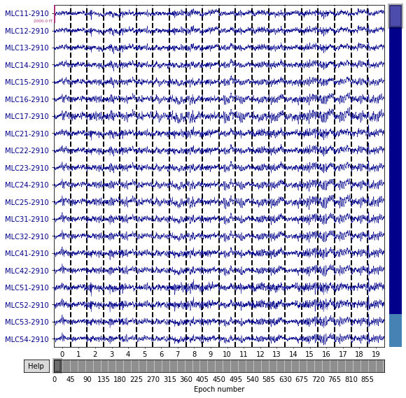
The panel each contains 900 epochs. In these samples, there are no spikes or other distinctive abnormal waveforms. For every single training dataset from various participants, 900 of in total 900 events passed the rejection process. It is because the rejection algorithm was purposefully designed to be inclusive. All data were deliberately included because the CNN model should be robust to noise in the data

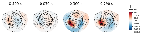
Topological map from -500.00 to 790.00 ms. The brain areas that are activated are concentrated in the downstream temporal region or visual cortex.

A few questions at last:

why do we split the data as 70%, does it work as other ration?

Because we have got enough data to train and need more data to test and valid the training performance.

April 26th

MRI safety training for 2.5 hrs

update Anaconda (start to use a new platform)

Anaconda is a good environment manager tool which allows me to manage and deploy packages

conda update conda

conda update anaconda

conda update --all

done

Python version: 3.8.13-h6244533_0

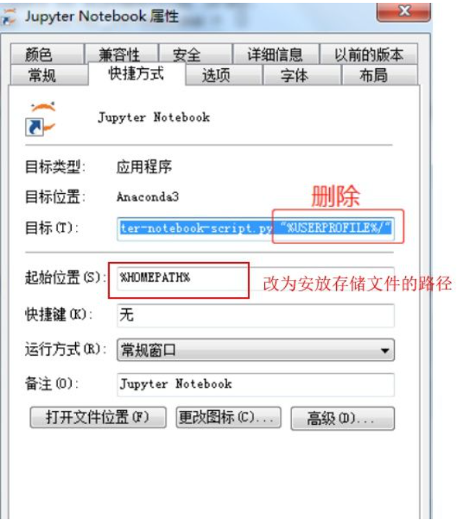
change the directory path of Jupyter notebook (in order to save files in preferred path)

jupyter notebook --generate-config get the config file. change the line c.NotebookApp.notebook_dir = '' to the directory I want
find jupyter notebook file, change the attributes.

Link the local directory and Github

for the convenience of collaboration

SSH connect public key (id_rsa.pub) was created before.

after create the directory, run the command in git:

git init
git add .
git git commit -m  "Comment"
git remote add origin "the url of directory"
git push -u origin main

Journal club preparation for the next session

April 27th

Pycharm (use IDE)

Get Pycharm educational version via King’s email

install python 3.8 environment for running the code from https://github.com/tobywise/aversive_state_reactivation (because it was coding with python 3.8 compiler)

run below code in pycharm

!conda create -n py38 python=3.8
!pip install mne
!pip install scikit-learn
!pip install plotly
!pip install cufflinks
!pip install networkx
!conda install numba
!pip install pyyaml
!pip install papermill

Fixation for some expired code

The function joblib does not exist in sklearn.external anymore.

Error occurs when run the function plot_confusion_matrix:

Deprecated since version 1.0: plot_confusion_matrix is deprecated in 1.0 and will be removed in 1.2. Use one of the following class methods: from_predictions or from_estimator.

use

ConfusionMatrixDisplay.from_predictions(y, y_pred)

instead of

plot_confusion_matrix(mean_conf_mat[:n_stim, :n_stim], title='Normalised confusion matrix, accuracy = {0}'.format(np.round(mean_accuracy, 2)))

Second session meeting

Every people gives a general introduction of their projects

April 28th

Logistic regression cost function

The function is using the principle of maximum likelihood estimation to find the parameters $\theta$ for different models. At the meantime, a nice property is it is convex. So, this cost function is generally everyone use for fitting parameters in logistic regression.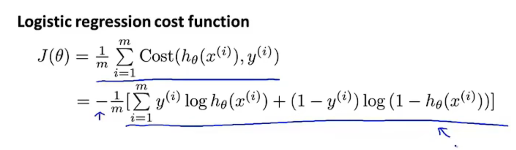

The way we are going to minimize the cost function is using gradient descent:

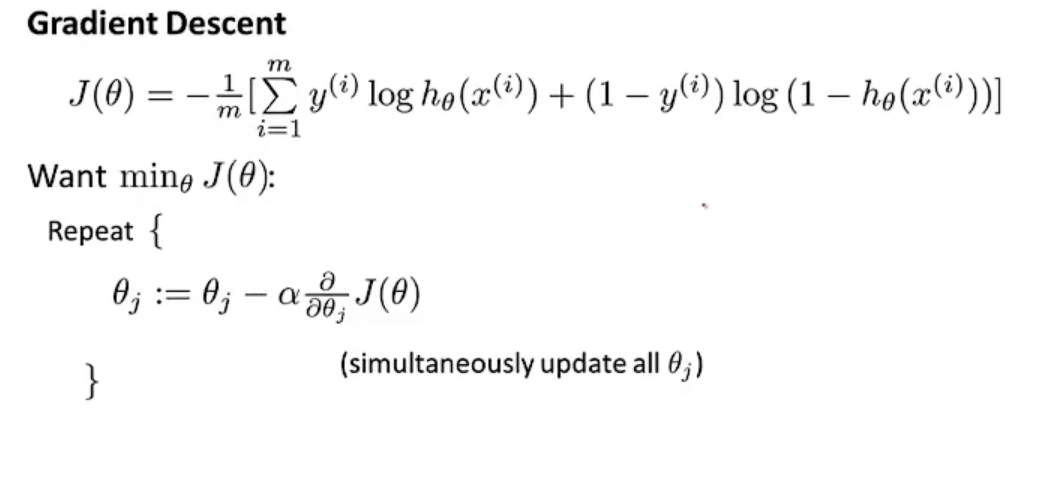
Other alternative optimization algorithms (no need to manually pick $\alpha$ studying rate):

Conjugate gradient
BFGS
L-BFGS

Methods to storage trained model

set and train a simple SVC model

from sklearn import svm
from sklearn import datasets

clf = svm.SVC()
iris = datasets.load_iris()
X, y = iris.data, iris.target
clf.fit(X,y)

Storage:

pickle

import pickle #pickle module

#store Model(Note: The save folder must be created in advance, otherwise an error will be reported)
with open('save/clf.pickle', 'wb') as f:
    pickle.dump(clf, f)

#load Model
with open('save/clf.pickle', 'rb') as f:
    clf2 = pickle.load(f)
    #test loaded Model
    print(clf2.predict(X[0:1]))

joblib (supposed to be faster when dealing with a large data, because the use of multiprocessing)

from sklearn.externals import joblib #jbolib模块

#store Model(Note: The save folder must be created in advance, otherwise an error will be reported)
joblib.dump(clf, 'save/clf.pkl')

##load Model
clf3 = joblib.load('save/clf.pkl')

#test loaded Model
print(clf3.predict(X[0:1]))

April 29th

Google Colab

Get the subscription of Google Colab and Google drive

clone data to google drive

Token: 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

connect Google Colab with VS code

Regularization

We can use regularization to rescue the overfitting

There are two types of regularization:

L1 Regularization (or Lasso Regularization)

$Min$($$\sum_{i=1}^{n}{|y_i-w_ix_i|+p\sum_{i=1}^{n}|w_i|}$$)
L2 Regularization (or Ridge Regularization)

$Min$($$\sum_{i=1}^{n}{(y_i-w_ix_i)^2+p\sum_{i=1}^{n}w_i^2}$$)

where p is the tuning parameter which decides in what extent we want to penalize the model.

However, there is another method for combination

Elastic Net: When L1 and L2 regularization combine together, it becomes the elastic net method, it adds a hyperparameter.

how to select:

No	L1 Regularization	L2 Regularization
1	Panelises the sum of absolute value of weights.	Penalises the sum of square weights.
2	It has a sparse solution.	It has a non-sparse solution.
3	It gives multiple solutions.	It has only one solution.
4	Constructed in feature selection.	No feature selection.
5	Robust to outliers.	Not robust to outliers.
6	It generates simple and interpretable models.	It gives more accurate predictions when the output variable is the function of whole input variables.
7	Unable to learn complex data patterns.	Able to learn complex data patterns.
8	Computationally inefficient over non-sparse conditions.	Computationally efficient because of having analytical solutions.

Normalization

The reason for applying normalization is the normalization step can generalize the statistical distribution of uniform samples, which is expected to enhance the training performance.

where m is the total number of data and x represents data, makes the average value and standard deviation of data in each channel to be located in the range between 0 and 1

Question:

which layer should I apply the regularization?

From the model’s summary, I can determine which layers have the most parameters. It is better to apply regularization to the layers with the highest parameters.

In the above case, how to get each layer’s parameters?

from prettytable import PrettyTable

def count_parameters(model):
    table = PrettyTable(["Modules", "Parameters"])
    total_params = 0
    for name, parameter in model.named_parameters():
        if not parameter.requires_grad: continue
        params = parameter.numel()
        table.add_row([name, params])
        total_params+=params
    print(table)
    print(f"Total Trainable Params: {total_params}")
    return total_params

count_parameters(model)

May 2nd

Question ahead:

get a question: how to determine the classifier centre (windows width)?

for this case, it is around 20 to be at the middle/ top

GPU accelerations

It could be a little bit tricky to accelerate the calculation in sklearn with GPU. Here is a possible solution: https://developer.nvidia.com/blog/scikit-learn-tutorial-beginners-guide-to-gpu-accelerating-ml-pipelines/.

Third meeting:

Deep learning might be the solution for MEG signals classification.

The CNN is a particular subtype of the neural network, which is effective in analysing images or other data containing high spatial information (Khan et al., 2018; Valueva et al., 2020) and also works well with temporal information (Bai et al., 2018)

Khan, S., Rahmani, H., Shah, S. A. A., & Bennamoun, M. (2018). A Guide to Convolutional Neural Networks for Computer Vision. A Guide to Convolutional Neural Networks for Computer Vision. https://doi.org/10.1007/978-3-031-01821-3

Valueva, M. v., Nagornov, N. N., Lyakhov, P. A., Valuev, G. v., & Chervyakov, N. I. (2020). Application of the residue number system to reduce hardware costs of the convolutional neural network implementation. Mathematics and Computers in Simulation, 177, 232–243. https://doi.org/10.1016/J.MATCOM.2020.04.031

Bai, S., Kolter, J. Z., & Koltun, V. (2018). An Empirical Evaluation of Generic Convolutional and Recurrent Networks for Sequence Modeling. https://doi.org/10.48550/arxiv.1803.01271

possible deep learning packages:

JAX, HAIKU

My aim is to inform bad-performance data with the training model of good-performance data in aims to increase the performance. One hallmark is to increase the mean accuracy of each cases as high as possible.

May 3rd

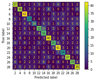
Successfully run the code for confusion matrix.

clf.set_params(**random_search.best_params_)

# Get predictions with 5 fold CV
y_pred = cross_val_predict(clf, X, y, cv=confusion_matrix_cv)
mean_conf_mat = confusion_matrix(y, y_pred)
mean_accuracy = accuracy_score(y[y != 99], y_pred[y != 99])
mean_conf_mat = mean_conf_mat.astype('float') / mean_conf_mat.sum(axis=1)  # normalise

print("Mean accuracy = {0}".format(mean_accuracy))

# Plot mean confusion matrix
#plot_confusion_matrix(mean_conf_mat[:n_stim, :n_stim], title='Normalised confusion matrix, accuracy = {0}'.format(np.round(mean_accuracy, 2)))
#plt.imshow(mean_conf_mat[:n_stim, :n_stim])

ConfusionMatrixDisplay.from_predictions(y, y_pred)
plt.savefig('./save_folder/fig-{}.png'.format(session_id), dpi=600)
plt.show()

pictures of each case are stored in the Github depository:

https://github.com/ReveRoyl/MT_ML_Decoding/tree/main/Aversive_state_reactivation/notebooks/templates/save_folder

It takes around 36 minutes to run 28 cases.

Mean accuracy with existing code:

[0.4288888888888889, 0.33666666666666667, 0.2777777777777778, 0.5022222222222222, 0.5066666666666667, 0.4245810055865922, 0.5577777777777778, 0.43222222222222223, 0.65, 0.47888888888888886, 0.3377777777777778, 0.4800469483568075, 0.27111111111111114, 0.37193763919821826, 0.4288888888888889, 0.40555555555555556, 0.46444444444444444, 0.7077777777777777, 0.5811111111111111, 0.4711111111111111, 0.4255555555555556, 0.5022222222222222, 0.45394006659267483, 0.38555555555555554, 0.6222222222222222, 0.4622222222222222, 0.35444444444444445, 0.47444444444444445]

May 10th

Get rid of the effect of null data

transform X into the same size as clf

May 11th

Grid Search CV

To test Grid Search CV instead of Randomized Search CV

However, the result of grid search CV is worse than the randomized search CV. I think the reason is that random search CV uses a random combination of hyperparameters to find the best solution for a built model. However, the random search CV is not 100% better than grid search CV: the disadvantage of random search is that it produces high variance during computation.

Concatenation

Objective

Since my aim is to transfer the model prediction of one case to anther, I try to concatenate multiple cases data together to train the model and see what will happen.

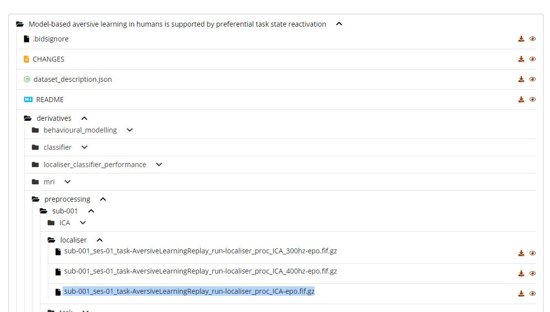
localiser_epochs = mne.read_epochs(os.path.join(output_dir, 'preprocessing', 'sub-{}', 'localiser', 'sub-{}_ses-01_task-AversiveLearningReplay_run-localiser_proc_ICA-epo.fif.gz').format('001','001')) 

for session_id_int in range(2, 3):
    session_id = '{:03d}'.format(session_id_int)
    print(session_id)

    localiser_epochs_unconcatenate = mne.read_epochs(os.path.join(output_dir, 'preprocessing', 'sub-{}', 'localiser', 'sub-{}_ses-01_task-AversiveLearningReplay_run-localiser_proc_ICA-epo.fif.gz').format(session_id,session_id))  
    localiser_epochs_unconcatenate.info = localiser_epochs.info
    localiser_epochs = mne.concatenate_epochs([localiser_epochs, localiser_epochs_unconcatenate])

Result

Concatenate X np arrays and test, the mean accuracy increases. I test 5 cases.

Mean accuracy = 0.5111111111111111, while for each cases, previous mean accuracy = 0.43777777777777777; 0.34; 0.2788888888888889; 0.5055555555555555.

The concatenated data gives a better fit:

output

However, the generalization ability of this method has not been decided yet till now.

May 12th

add ‘participant number’ dimension to X

X_4D = []
for session_id_int in range(1, 2):
    session_id = '{:03d}'.format(session_id_int)
    print(session_id)
    # Get data
    localiser_epochs = mne.read_epochs(os.path.join(output_dir, 'preprocessing', 'sub-{}', 'localiser', 'sub-{}_ses-01_task-AversiveLearningReplay_run-localiser_proc_ICA-epo.fif.gz').format(session_id,session_id))  

    X_raw = localiser_epochs.get_data()

    picks_meg = mne.pick_types(localiser_epochs.info, meg=True, ref_meg=False)
    event_selector = (y_raw < n_stim * 2 + 1)
    X_raw = X_raw[event_selector, ...]
    X_raw = X_raw[:, picks_meg, :]
    X = X_raw.copy()
    X = X[..., classifier_center_idx + classifier_window[0]:classifier_center_idx + classifier_window[1]] 

    X_4D.append(X)
# for epoch in localiser_epochs_concatenate:
#     print(epoch.shape)
# localiser_epochs = mne.concatenate_epochs(localiser_epochs_concatenate)
X = np.stack(X_4D)

It takes me 1 hour to make the code logical elegant.

May 13th

Forth meeting

Objective:

We have tested existing code, the following step is to try different models to predict.

My supervisor’s suggestion is to use haiku trying CNN.

pip install -upgrade jax optax dm-haiku

to be learnt:

active function: rectifier RELU

Result:

New model selection: CNN with Haiku

May 14th

Find a bug: concatenated data was not giving a correct result. The better performance was because of the randomness of every time training. The concatenated data won’t give a better prediction.

possible solution: transfer learning instead of directly concatenation.

May 16th

Objective

to learning deep learning courses (Andrew Ng) in coursera because as said in ‘Knife don’t miss your job’, to solid the foundation of deep learning will help me build the CNN and understand others’ work

Result:

In the context of artificial neural networks, the rectifier or ReLU (Rectified Linear Unit) activation function is an activation function defined as the positive part of its argument.

Convolution

Types of layer in a CNN:

Covolution
Pooling
Fully connected

Cases:

Classic networks:

LeNet-5
AlexNet
VGG

ResNet

Inception

LeNet -5

May 17th

Learning JAX

Question: why jax has its own numpy type: jax.numpy? what is the difference between it and numpy?

Jax.numpy is a little bit different from numpy: the former is immutable

Question: why do we need jax.numpy?

because numpy only works on CPU while jax.numpy works on GPU

another advantage of JAX

jit() can be used to compile the data input thus makes the program run faster

First group meeting

Yiqi introduced his recent work which is based on U-net, VAE

May 18th

Learning JAX

grad() # for differentation
from jax import jacfwd, jacrev # for Jacobian matrix
vmap() # for vectorization; it can makes you write your functions as if you were dealing wiht a single datapoint

JAX API structure

NumPy <-> lax <-> XLA
lax API is stricter and more powerful
It’s a Python wrapper around XLA

class CNN(hk.Module):
    def __init__(self):
        super().__init__(name="CNN")
        # self.conv1 = hk.Conv2D(output_channels=32, kernel_shape=(3,3), padding="SAME")
        # self.conv2 = hk.Conv2D(output_channels=16, kernel_shape=(3,3), padding="SAME")
        self.conv1 = hk.Conv2D(output_channels=64, kernel_shape=(11,11), stride=4, padding="SAME")
        self.conv2 = hk.Conv2D(output_channels=192, kernel_shape=(5,5), padding="SAME")
        self.conv3 = hk.Conv2D(output_channels=384, kernel_shape=(3,3), padding="SAME")
        self.conv4 = hk.Conv2D(output_channels=256, kernel_shape=(3,3), padding="SAME")
        self.conv5 = hk.Conv2D(output_channels=256, kernel_shape=(3,3), padding="SAME")
        self.flatten = hk.Flatten()
        self.linear = hk.Linear(len(classes))

    def __call__(self, x_batch):
        x = self.conv1(x_batch)
        x = jax.nn.relu(x)
        x = hk.MaxPool(window_shape=(3, 3), strides=(2, 2), padding='VALID')(x)
        x = self.conv2(x)
        x = jax.nn.relu(x)
        x = hk.MaxPool(window_shape=(3, 3), strides=(2, 2), padding='VALID')(x)        
        x = self.conv3(x_batch)
        x = jax.nn.relu(x)
        x = self.conv4(x_batch)
        x = jax.nn.relu(x)
        x = self.conv5(x_batch)
        x = jax.nn.relu(x)
        x = hk.MaxPool(window_shape=(3, 3), strides=2, padding='VALID')(x)
        # x = hk.AvgPool(window_shape=(6, 6), strides=(2, 2), padding='SAME')(x)

        x = self.flatten(x)
        x = self.linear(x)
        x = jax.nn.softmax(x)
        return x

May 19th

Test CNN

CNN test was run but the prediction result is not as good as expected:

the performance of it is about 0.4 for training dataset and 0.15 for test dataset.

I think we should try to tune the parameters of model or test a different model since the current model is suitable for image recognition. Before that, literature reviews should be done.

Later after I read Aoe’s work, I start to under stand it is because my image classification CNN model fails to extract the temporal and spatial information.

Aoe, J., Fukuma, R., Yanagisawa, T., Harada, T., Tanaka, M., Kobayashi, M., Inoue, Y., Yamamoto, S., Ohnishi, Y., & Kishima, H. (2019). Automatic diagnosis of neurological diseases using MEG signals with a deep neural network. Scientific Reports, 9(1). https://doi.org/10.1038/S41598-019-41500-X

Fifth meeting

I have the requirement of visualization during training:

To use Tensor Board to show the training process

!rm -rf /logs/ # clear logs
# if 'google.colab' in str(get_ipython()): # tensor board
%load_ext tensorboard  
# %tensorboard --logdir logs
%tensorboard --logdir=./models/test

May 20th

Tried AlexNet (can be easily get from Pytorch hub)

AlexNet

AlexNet  = torch.hub.load('pytorch/vision:v0.10.0', 'alexnet', pretrained=True).cuda()

Resnet 18

Resnet   = torch.hub.load('pytorch/vision:v0.10.0', 'resnet18', pretrained=True).cuda()

These 2 models fail as well. The same reason: these models fail to extract the temporal and spatial information in the first convolutional layers.

Sixth meeting

Objective:

to discuss about that if we should use concatenate data and pre-processing for standardization because the conditions of recording may varies a lot among different subjects: the device position or potential individual reasons.

Results:

Dr. Toby and I had a discussion together with Dr. Rossalin

Rossalin advices me to try transfer learning or LSTM.

After trying the model is usually used in image classification, it is a good idea to try the model LSTM RNN, which is known as a good fit for sequential data.

May 24th

Second group meeting

Zarc gives a presentation about his NLP project.

May 27th

Learning Tensorflow

Tensorflow is a more popular packages which allows me to get access to many templates. Some research is also using Tensorflow as their machine learning library. But I found Pytorch is a more popular packages which allows me to get access to more well-known templates. Most related research is using Pytorch as their machine learning library.

However, I found the variable and placeholder operations are more commonly used in Tensorflow-v1 rather than the latest Tensorflow-v1

Session control

In Tensorflow, a string is defined as a variable, and it is a variable, which is different from Python. (later on I found it was correct in Tensorflow v1 but changes in Tensorflow v2)

state = tf.Variable()

import tensorflow as tf

state = tf.Variable(0, name='counter')

# define variable one
one = tf.constant(1)

# define plus step (hint: no computation here)
new_value = tf.add(state, one)

# update State to new_value
update = tf.assign(state, new_value)

If I set variables in Tensorflow, initializing the variables is the most important thing! ! So after defining the variable, be sure to define init = tf.initialize_all_variables().

At this point, the variable is still not activated, and it needs to be added in sess , sess.run(init) , to activateinit. (again, it changes in v2, we do not need to initialize the session in Tensorflow v2)

# Variable, initialize
# init = tf.initialize_all_variables() # expired
init = tf.global_variables_initializer()  

# Session
with tf.Session() as sess:
    sess.run(init)
    for _ in range(3):
        sess.run(update)
        print(sess.run(state))

Note: directly print(state) does not work! !

Be sure to point the sess pointer to state and then print to get the desired result!

placeholder

placeholder is a placeholder in Tensorflow that temporarily stores variables.

If Tensorflow wants to pass in data from the outside, it needs to use tf.placeholder(), and then transfer the data in this form sess.run(***, feed_dict={input: **}).

Examoles：

import tensorflow as tf

# Tensorflow requires defining placeholder's type, usually float32
input1 = tf.placeholder(tf.float32)
input2 = tf.placeholder(tf.float32)

# multiply input1 and input2
ouput = tf.multiply(input1, input2)

Next, the work of passing the value is handed over to sess.run(), the value that needs to be passed in is placed in feed_dict={} and corresponds to each input one by one. placeholder and feed_dict={ } are bound together.

with tf.Session() as sess:
    print(sess.run(ouput, feed_dict={input1: [7.], input2: [2.]}))
# [ 14.]

Activation function

when there are many layers, be careful to use activation function in case of the gradient exploding or gradient disappearance.

May 28th

Although in the computer vision field convolutional layer often followed by a pooling layer to reduce the data dimension at the expense of information loss, in the scenes of MEG decoding, the size of MEG data is much smaller than the computer vision field. So in order to keep all the information, we don’t use the pooling layer. After the spatial convolutional layer, we use two layers of temporal convolutional layers to extract temporal features, a fully connected layer with dropout operation for feature fusion, and a softmax layer for final classification. (Huang2019)

It is important to select if we should use pooling layers and how many to use.

May 30th

ML optimizer

Objective:

to learn how to use and select different optimizer, because it modifies model’s parameters like weights and learning rate, which helps to increase accuracy and reduce overall loss.

Results:

Stochastic Gradient Descent (SGD)
Momentum
AdaGrad
RMSProp
Adam

speedup3

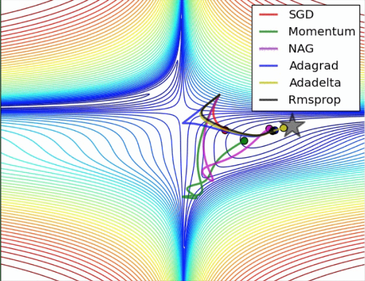
X.shape gives (n_epochs, n_channels, n_times) corresponding to (batches, pixels,channels) of images

Apart for optimizer, scheduler may help a lot with providing a dynamic learning rate.

impression

As I tried to apply regularization at the same time. It is important to bear in mind, if we give a momentum in SGD (about 0.9), we can easily apply L2 regularization when the weight_decay is larger than 0.

May 31st

Objective:

to learn data augmentation and learn a important rule: “No free lunch theorem”

Results:

D. H. Wolpert et. al. (1995) come up with “No free lunch theorem”: all optimization algorithms perform equally well when their performance is averaged across all possible problems.

For any prediction function, if it performs well on some training samples, it must perform poorly on other training samples. If there are certain assumptions about the prior distribution of the data in the feature space, there are as many good and bad performances.

Later I found relative power spectrum including delta (0.5-4 Hz), theta (4-8 Hz), alpha (8-12 Hz), beta (12-30Hz), and gamma (above 30 Hz), provide important information to augmenting the MEG data.

X_train_numpy = X_train_tensors.cpu().numpy()
X_test_numpy = X_test_tensors.cpu().numpy()

X = np.swapaxes(X_train_numpy, 2, -1).squeeze()
data = X[X.shape[0]-1, 70, :]
psd_mne, freqs_mne = psd_array_welch(data, 100, 1., 70., n_per_seg=None,
                          n_overlap=0, n_jobs=1)
for low, high in [(0.5, 4), (4, 8), (8, 10), (10, 12), (12, 30),
                  (30, 70)]:
    print("processing bands (low, high) : ({},{})".format(low, high))
    # Find intersecting values in frequency vector
    idx_delta = np.logical_and(freqs_mne >= low, freqs_mne <= high)
      # Frequency resolution
    freq_res = freqs_mne[1] - freqs_mne[0]  # = 1 / 4 = 0.25

    # Compute the absolute power by approximating the area under the curve
    power = simps(psd_mne[idx_delta], dx=freq_res)
    print('Absolute power: {:.4f} uV^2'.format(power))

    total_power = simps(psd_mne, dx=freq_res)
    rel_power = power / total_power

    print('Relative power: {:.4f}'.format(rel_power))

Jun 1st

Seventh meeting

Dr Toby provide me the code to load data with dataloader

it defines load_MEG_dataset function with following parameters:

def load_MEG_dataset(
        subject_ids: List[str],
        mode: str = "individual",
        output_format: str = "numpy",
        trial_data_format: str = "2D",
        data_location: str = "./data/",
        center_timepoint: int = 20,
        window_width: List[int] = [-400, 400],
        shuffle: bool = False,
        pca_n_components: int = None,
        training: bool = True,
        train_test_split: float = 0.75,
        batch_size: int = 32,
        scale: bool = True,
        seed: int = 0,
    )

Jun 6th

Objective:

to try different loss function, because different evaluating methods may affect the learning process, and lead to a different approach to training results.

Results:

when apply other loss function instead of CrossEntropy, there are some format error occurs:

solution: transform inputs from multi hot coding into one hot coding.

def onehot(batches, n_classes, y):
  yn = torch.zeros(batches, n_classes)
  for i in range(batches):
    x = [0 for j in range(batches)]
    x[i] = y[i]/2-1                     #ex. [12]-> [5]
    yn[i][int(x[i])]+= 1                  #[000010000]
  return yn

Later I found that we can use the function in Pytorch: F.onehot

Jun 7th

try different models, reshape the data from [batches, channels, times point ]to be [batches, times point, channels] in corresponding to images format [batches, picture channels (layers), pixels] (not the same channels, the same names but different meanings, former one is electrode channels. latter one is picture layers)

Jun 8th

Third session meeting

Objective:

to learn the key points of writing a good introduction

Results:

from the history of ML to the current meaning

The history of ML, (black box…)
the history of disease classification or behaviour prediction
how people use the ML techniques to predict behaviours these days
what is aversive state reactivation (one sentence); why people want to learn aversive state reactivation
how people tried to connect ML with aversive state reactivation
the problem (gap) is previous model only gives a low prediction accuracy
Introduction of CNN, LSTM, RNN or transfer learning
My aims is to optimize the model with new techniques: CNN, LSTM RNN or transfer learning

Note: state what in each paragraph is not enough and leads to the next paragraph.

LSTM RNN

Objective:

try LSTM RNN

Results:

The problems when I try to use one hot data labels = F.one_hot(labels), it is not applicable because in that case the dimensions could be 28 instead of 14 as we only have even numbers,

Some packages automatically figure out where there missing labels during one hot operation but this one (pytorch) doesn’t

Eighth meeting

questions:

loss functions give similar values?
~~is it correct to use enumerate to loop each data?~~

In my case, CrossEntropy is the better for MEG data. It is the experience gained from Dr Toby. Even though I found the others’ research about hands behaviour prediction used MSE loss. It is not suitable for our results because theirs is about the movements while ours is not.

Jun 9th

Label noise.

Objectives:

to figure out if labels format it self may affect the model performance. Because some models only accept data in one kind of format.

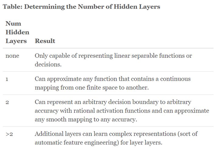
question: how to determine numbers of hidden layers in LSTM RNN.

Results:

We cannot correctly compare each label when we are using one-hot format. If the labels you predict are apples, bananas, and strawberries, obviously they do not directly have a comparison relationship. If we use 1, 2, 3 as labels, there will be a comparison relationship between the labels. Distances are different. With the comparison relationship, the distance between the first label and the last label is too far, which affects the learning of the model.

One promotion:

Knowledge distillation (KD) improves performance precisely by suppressing this label nosie. Based on this understanding, we introduce a particularly simple improvement method of knowledge disillation, which can significantly improve the performance of ordinary KD by setting different temperatures for each image.

Xu, K., Rui, L., Li, Y., Gu, L. (2020). Feature Normalized Knowledge Distillation for Image Classification. In: Vedaldi, A., Bischof, H., Brox, T., Frahm, JM. (eds) Computer Vision – ECCV 2020. ECCV 2020. Lecture Notes in Computer Science(), vol 12370. Springer, Cham. https://doi.org/10.1007/978-3-030-58595-2_40

Hidden layers in LSTM RNN

The effect of the number of hidden layers for neural networks

Jun 10th

try CrossEntropyLoss() with onehot format data

convert the labels from “every 2 in 0 to 28” to “every 1 in 1 to 14”

y_train = (y_train / 2) - 1
y_test = (y_test / 2) - 1

use with torch.autocast('cuda') to solve “cuda error” of CrossEntropyLoss()

with torch.autocast('cuda'):
        # loss = criterion(outputs, torch.tensor(labels).cuda())
            loss = criterion(outputs, labels)

Jun 12th

even though the accuracy of prediction for train data increases quickly as training, the accuracy for test data is still very low. It seems the validation loss does not converge. I decide the next step is going to do more literature research and adjust the parameters.

Jun 13th

Problems:

the problem is overfitting. There could be 2 alternative options: 1, get more data; 2, try different learning rate or dynamic learning rate.

the way the train-test split worked wasn’t ideal in the data loading function - because the data wasn’t shuffled prior to splitting, the train and test set would often consist of different subjects if we load multiple subjects. The data can be shuffled before splitting (by setting shuffle=True), which means that there will be a mix of subjects in both the training and testing data. This seems to boost accuracy in the test set a little bit.

Jun 14th

Objective:

to try CosineEmbeddingLoss() because it is reported that cosine loss may improve the performance for small dataset

Cosine loss could have better performance for small dataset (around 30%).

Barz, B., & Denzler, J. (2019). Deep Learning on Small Datasets without Pre-Training using Cosine Loss. Proceedings - 2020 IEEE Winter Conference on Applications of Computer Vision, WACV 2020, 1360–1369. https://doi.org/10.48550/arxiv.1901.09054

Results:

however, the performance is not promoted

Jun 15th

Fourth session meeting

I read others work, practice to extract the key words and main ideas:

Affective modulation of the startle response in depression: Influence of the severity of depression, anhedonia and anxiety

startle reflex (SR)

affective rating

get affective rating after participants watched every clips

and analysis the difference between depressed patients and control.

Startle amplitude
EMG

higher baseline EMG activity during pleasant and unpleasant clips, relative to the neutral clips

Conclusion

a reduced degree of self-reported mood modulation

Gap

The findings differ from those of Allen et al. (1999): they think it does not matter for depression or anhedonia for affective and emotional modulation.

key wards

Depression

Anxiety

Anhedonia

Affective modulation

Mood regulation

Startle response

EMG

affective rating

Ninth meeting

Problems:

Since the past work does not give a good result and it has been nearly halfway of the project. My following work is suggested to be focused on:

Multilayer Perceptron
transfer learning

Jun 16th

Convolutional Layer : Consider a convolutional layer which takes “l” feature maps as the input and has “k” feature maps as output. The filter size is “n*m”.
Here the input has l=32\ feature maps as inputs, k=64\ feature maps as outputs and filter size is n=3 and m=3\. It is important to understand, that we don’t simply have a 33 filter, but actually, we have *3*3*32** filter, as our input has 32 dimensions. And as an output from first conv layer, we learn 64 different 3*3*32 filters which total weights is “n*m*k*l”. Then there is a term called bias for each feature map. So, the total number of parameters are “(n*m*l+1)*k”.

https://medium.com/@iamvarman/how-to-calculate-the-number-of-parameters-in-the-cnn-5bd55364d7ca

bicubic interpolation: torch.nn.functional.interpolate() with mode=’bicubic’

https://stackoverflow.com/questions/54083474/bicubic-interpolation-in-pytorch

Meeting these data and fitting problems, I realize the insufficiency of understanding data itself, so I look back to the Machine Learning courses materials from 2 years ago, trying to get some new approaches.

When reading the Chapter 1 of Computational Modelling of Cognition and Behaviour, I get the following points:

Data never speak for themselves but require a model to be understood and to be explained.

Verbal theorizing alone ultimately cannot replace for quantitative analysis.

There are always several alternative models that vie for explanation of data and we must select among them.

Model selection rests on both quantitative evaluation and intellectual and scholarly judgment.

June 21th

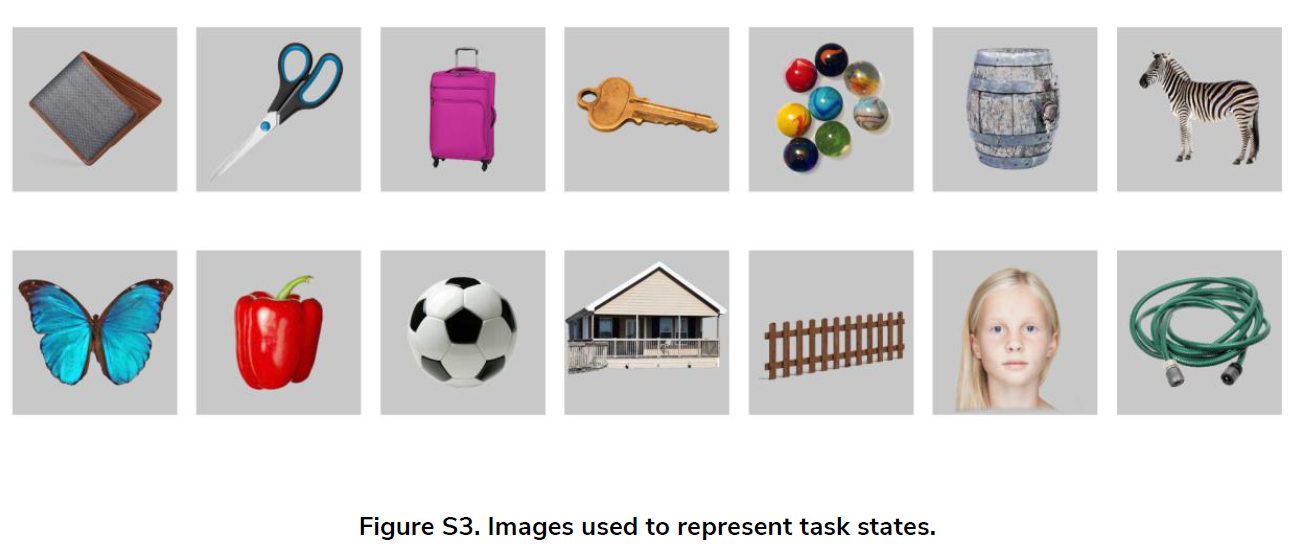
Have a meeting with Eammon, we talked about my recent work:

Eammon gives me a suggestion: in behaviour level, picture of faces are different. Try and see what if we get rid of the picture of faces in labels.

Here are the pictures shown to participants:

June 25th

to try Mnet (was used to predict the Alzheimer’s disease by Aoe .etc)

Aoe, J., Fukuma, R., Yanagisawa, T. et al. Automatic diagnosis of neurological diseases using MEG signals with a deep neural network. Sci Rep 9, 5057 (2019). https://doi.org/10.1038/s41598-019-41500-xz

Score method:

As an alternative option, the accuracy can be expressed as root mean square error.

Jun 27th

Objective:

to apply data augmentation because it was reported that relative power spectrum provide extra information which may improve model’s performance on MEG data.

Result:

one possible solution is to extract band power to augment the data

“This model was implemented to check the proprieties of the RPS to extract meaningful features from the input data. The RPS was combined with an MLP to add nonlinearity and increase the capability of approximate the target variable.”

The RPS was implemented in 4 steps:

Compute the modified periodogram using Welch methods (Welch 1967) to get the power spectral density.

Calculate the average band power approximating using the composite Simpson’s rule to get it for a specific target band.

Divide the average band power of the specific target band by the total power of the signal to get the relative power spectrum.

Anelli, M. (2020). Using Deep learning to predict continuous hand kinematics from Magnetoencephalographic (MEG) measurements of electromagnetic brain activity (Doctoral dissertation, ETSI_Informatica).

X_train_bp = np.squeeze(X_train_numpy, axis=1)
# X_train_bp = X_train_bp[: :, :, :]
X_train_bp = standard_scaling_sklearn(X_train_bp)
X_test_bp = np.squeeze(X_test_numpy, axis=1)
# X_train_bp = X_train_bp[: :, :, :]
X_test_bp = standard_scaling_sklearn(X_test_bp)
bands = [(1, 4), (4, 8), (8, 10), (10, 13), (13, 30), (30, 70)]
bp_train = bandpower_multi_bands(X_train_bp, fs=800.0, bands=bands, relative=True)
bp_test = bandpower_multi_bands(X_test_bp, fs=800.0, bands=bands, relative=True)
bp_train_tensor = torch.Tensor(bp_train).cuda()
bp_test_tensor = torch.Tensor(bp_test).cuda()

June 28th

Problem:

My Google Colab subscriptions is expired but luckily I have got the access of HPC in KCL (create)

Solution:

set up cluster as the tutorial: https://docs.er.kcl.ac.uk/CREATE/access/

Start an interactive session:

srun -p gpu --pty -t 6:00:00 --mem=30GB --gres=gpu /bin/bash

Make a note of the node I am connected to, e.g. erc-hpc-comp001

sinfo avail to check the available cores

start Jupyter lab without the display on a specific port (here this is port 9998)

jupyter lab --no-browser --port=9998 --ip="*"

Open a separate connection to CREATE that connects to the node where Jupyter Lab is running using the port you specified earlier. (Problems known with VScode terminal)

ssh -m hmac-sha2-512 -o ProxyCommand="ssh -m hmac-sha2-512 -W %h:%p k21116947@bastion.er.kcl.ac.uk" -L 9998:erc-hpc-comp031:9998 k21116947@hpc.create.kcl.ac.uk

Note:
- k12345678 should be replaced with your username.
- erc-hpc-comp001 should be replaced with the name of node where Jupyter lab is running
- 9998 should be replaced with the port you specified when running Jupyter lab (using e.g. --port=9998)
- authorize via https://portal.er.kcl.ac.uk/mfa/

Start notebook in http://localhost:9998/lab
VS code part: set the Jupyter server as remote :
```
http://localhost:9998/lab?token=XXX
# replace the localhost as erc-hpc-comp031
```
Note: However, After the latest weekly update, existing problem has been found is the connection via VS code is not stable. Reason could be the dynamic allocated node and port confuses the VS code connection server.

June 29th

Objective:

to try different normalization method: Z-Score Normalization

Results:

which maps the raw data to a distribution with mean 0 and standard deviation

Assuming that the mean of the original feature is μ and the variance is σ , the formula is as follows:

July 1th

Objective:

to try Mnet with band power (RPS Ment); the reason for splitting alpha into low and high is that kinematic show that alpha band significant after movement and beta before movement. It is also reported that gamma band is associated with it is related to synergistic muscle activation (Kolasinski et. al, 2019)

Kolasinski, J., Dima, D. C., Mehler, D. M. A., Stephenson, A., Valadan, S., Kusmia, S., & Rossiter, H. E. (2019). Spatially and temporally distinct encoding of muscle and kinematic information in rostral and caudal primary motor cortex. BioRxiv, 613323. https://doi.org/10.1101/613323

Results:

extract band powers to get a 6 RPS (relative power spectrum) for each frequency period:

def bandpower_1d(data, sf, band, nperseg=800, relative=False):

    # band = np.asarray(band)
    low, high = band

    # Compute the modified periodogram (Welch)
    # TODO: generalize freq values
    psd, freqs = psd_array_welch(data, sf, 1., 70., n_per_seg=int(800 / 2),
                                 n_overlap=0, n_jobs=1)

    # Frequency resolution
    freq_res = freqs[1] - freqs[0]

    # Find closest indices of band in frequency vector
    idx_band = np.logical_and(freqs >= low, freqs <= high)

    # Integral approximation of the spectrum using Simpson's rule.
    bp = simps(psd[idx_band], dx=freq_res)

    if relative:
        bp /= simps(psd, dx=freq_res)
    return bp

def bandpower(x, fs, bands, nperseg=800, relative=True):

    psd, freqs = psd_array_welch(x, fs, 1., 70., n_per_seg=int(fs/2),
                                 n_overlap=0, n_jobs=1)
    # Frequency resolution
    freq_res = freqs[1] - freqs[0]
    n_channel, _ = x.shape
    bp = np.zeros((n_channel, len(bands)))
    for idx, band in enumerate(bands):
        low, high = band
        # Find closest indices of band in frequency vector
        idx_band = np.logical_and(freqs >= low, freqs <= high)

        # Integral approximation of the spectrum using Simpson's rule.
        _bp = simps(psd[..., idx_band], dx=freq_res, axis=-1)

        if relative:
            _bp /= simps(psd, dx=freq_res, axis=-1)

        # print(bp.shape, _bp.shape) #272,6  80,272
        bp[:, idx] = _bp

    return bp

def bandpower_multi_bands(x, fs, bands,  nperseg=800, relative=True):

    n_epoch, n_channel, _ = x.shape
    bp = np.zeros((n_epoch, n_channel, len(bands)))
    for e in range(n_epoch):
        bp[e] = bandpower(x[e], fs, bands, nperseg=nperseg, relative=relative)

    return bp

def standard_scaling_sklearn(data):

    n_epoch = data.shape[0]
    for e in range(n_epoch):
        scaler = skScaler()
        data[e, ...] = scaler.fit_transform(data[e, ...])

    return data

In main code:

X = np.swapaxes(X_train, 2, -1).squeeze()
data = X[X.shape[0]-1, 70, :]
psd_mne, freqs_mne = psd_array_welch(data, 250, 1., 70., n_per_seg=None,
                          n_overlap=0, n_jobs=1)
for low, high in [(1, 4), (4, 8), (8, 10), (10, 13), (13, 30),
                  (30, 70)]:
    print("processing bands (low, high) : ({},{})".format(low, high))
    # Find intersecting values in frequency vector
    idx_delta = np.logical_and(freqs_mne >= low, freqs_mne <= high)
      # Frequency resolution
    freq_res = freqs_mne[1] - freqs_mne[0]  # = 1 / 4 = 0.25

    # Compute the absolute power by approximating the area under the curve
    power = simps(psd_mne[idx_delta], dx=freq_res)
    print('Absolute power: {:.4f} uV^2'.format(power))

    total_power = simps(psd_mne, dx=freq_res)
    rel_power = power / total_power

    print('Relative power: {:.4f}'.format(rel_power))

```
Outputs:
Effective window size : 1.024 (s)
processing bands (low, high) : (1,4)
Absolute power: 0.0610 uV^2
Relative power: 0.1251
processing bands (low, high) : (4,8)
Absolute power: 0.0315 uV^2
Relative power: 0.0647
processing bands (low, high) : (8,10)
Absolute power: 0.0220 uV^2
Relative power: 0.0452
processing bands (low, high) : (10,13)
Absolute power: 0.0031 uV^2
Relative power: 0.0064
processing bands (low, high) : (13,30)
Absolute power: 0.0577 uV^2
Relative power: 0.1184
processing bands (low, high) : (30,70)
Absolute power: 0.2356 uV^2
Relative power: 0.4837
```

The average power spectrum for all subjects:

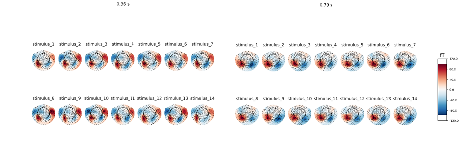
The results show that beta and delta waves are in the large and major proportion. It may be considered as potential evidence that beta and delta waves are associated with not only anxious thinking, and active concentration (Baumeister et al., 2013), but also the aversive state. In the following classifier task, these findings are in line with results showing the involvement of beta and delta in concentration.

Baumeister, J., Barthel, T., Geiss, K. R., & Weiss, M. (2013). Influence of phosphatidylserine on cognitive performance and cortical activity after induced stress. Http://Dx.Doi.Org/10.1179/147683008X301478, 11(3), 103–110. https://doi.org/10.1179/147683008X301478

Problems:

find the initial loss is too huge and does not change afterwards. Guess it is because of too large initial loss or wrongly loss.backward()

solution:

parameters of optimizer was set wrongly, fix it with model.parameters()

July 2th

Problems:

looking for solution to merge the function

guess I am meeting “dying ReLU” problem

July 5th

Objectives:

to try dynamic learning rate and interpolate 130 time points to be 800 time points without losing too much information.

Solution:

scheduler = torch.optim.lr_scheduler.ReduceLROnPlateau(optimizer, 'max')

scheduler.step(acc[-1]) #at last of each epoch training

the update step: I use the dynamic learning rate when the valid loss approaches a plateau (function 4, where represents learning decay and L represents valid loss).

Multilayer perceptron

interpolate https://pytorch.org/docs/stable/generated/torch.nn.functional.interpolate.html

Learning rate scheduling https://pytorch.org/docs/stable/optim.html

July 9th

In order to make the input data the same shape as required, I use resample function localiser_epochs.copy().resample(800, npad='auto') to upsamle the data

CBAM modules are added because the attention block is composed of 2 parts: the channel attention module and the spatial attention module. Two modules help model focus more on the important information: channel dimension and spatial dimension. First, for the channel attention module, input data process average pooling and max pooling separately, where the average pooling layer is used to aggregate spatial information and the max pooling layer is used to maintain more extensive and precise context information as images’ edges.

Attention in Deep Learning, Alex Smola and Aston Zhang, Amazon Web Services (AWS), ICML 2019

class SpatialAttention(nn.Module):
    def __init__(self):
        super(SpatialAttention, self).__init__()
        self.compress = ChannelPool()
        self.spatialAttention = nn.Sequential(
            nn.Conv2d(2, 1, 7, 7, padding=3), #padding = (7-1)/2
            )

    def forward(self, x):
        # print('x',x.shape)
        x = self.compress(x)
        x = self.spatialAttention(x)
        # scale = F.sigmoid(x)
        scale = torch.sigmoid(x)

        return x * scale

class Flatten_MEG(nn.Module):
    def forward(self, x):
        return x.view(x.size(0), -1)

class ChannelAttention(nn.Module):
    """
            Implementation of a channel attention module.
        """
    class Showsize(nn.Module):
        def __init__(self):
            super(ChannelAttention.Showsize, self).__init__()
        def forward(self, x):
            # print(x.shape)
            return x

    def __init__(self, shape, reduction_factor=16):

        super(ChannelAttention, self).__init__()

        _, in_channel, h, w = shape
        self.mlp = nn.Sequential(
            # self.Showsize(),
            Flatten_MEG(),
            # self.Showsize(),
            nn.Linear(in_channel, in_channel // reduction_factor),
            nn.ReLU(),
            nn.Linear(in_channel // reduction_factor, in_channel),
        )

    def forward(self, x):
        avg_pool = F.avg_pool2d( x, (x.size(2), x.size(3)), stride=(x.size(2), x.size(3)))
        max_pool = F.max_pool2d( x, (x.size(2), x.size(3)), stride=(x.size(2), x.size(3)))
        sum = self.mlp(avg_pool) + self.mlp(max_pool)
        scale = (
            torch.sigmoid(sum)
            .unsqueeze(2)
            .unsqueeze(3)
            .expand_as(x)
        )

        return x * scale

July 10th

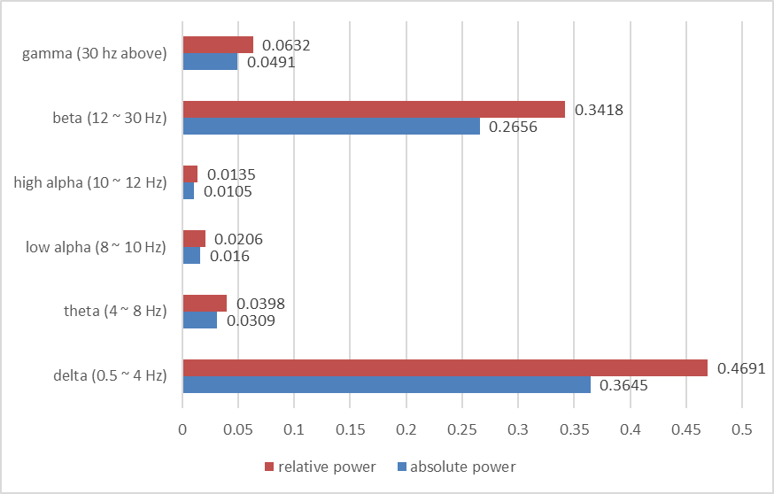
In order to find the rationality of extracting features of brain states under different stimuli. I draw the topographical maps of all stimuli at different time. It may suggest that stimulus representations are in the downstream temporal region or visual cortex. Thus, as the following training results showed, my model is an effective and reasonable approach to classifying these states.

sti=[1,2,3,4,5,6,7,8,9,10,11,12,13,14]                     
for stimuli in range (1,15):
    epochs_standard = fname.get_epochs(sub=1)
    for sub in [sub for sub in range (2,29) if sub not in [6, 12, 14 ,23]]:
        if sub == 1:
            epochs_standard = fname.get_epochs(sub=1)
        else:
            epochs = fname.get_epochs(sub)['stimulus_{}'.format(2*stimuli)]
            epochs.info['dev_head_t'] = epochs_standard.info['dev_head_t']
            epochs_standard = mne.concatenate_epochs([epochs_standard['stimulus_{}'.format(2*stimuli)], epochs['stimulus_{}'.format(2*stimuli)]])
    exec('evoked_{} = epochs_standard.average()'.format(stimuli))
        # evoked_standard = mne.concatenate_epochs([evoked_standard, evoked])

brain topographical map under different stimuli in the specific time (0.36 s, 0.79 s after giving the stimuli). The average brain states of all 24 subjects in all 14 stimuli are shown as the topographical map. The map shows these different brain states as an intensity map, where the red colour shows stronger intensity and blue shows weaker intensity.

July 12th

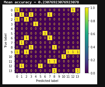
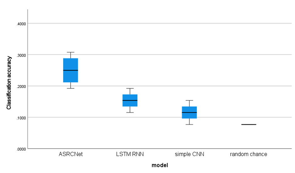
The random prediction accuracy is expected to be 7.14% (1/14 = 7.14%). The classification accuracy of my model is around 23.07%, which is clearly higher than random chance. LSTM RNN gives an accuracy of about 15.38% while simple CNN only gives a mean accuracy of 11.53%. Compared with the other classification approach, my model exhibits the best classification performance (p = 6.8 × 10 –2 for LSTM RNN, p = 5.9 × 10 –2 for CNN, paired Wilcoxon signed-rank tests). The best classification accuracy of my model is able to reach 33.33%.

early stopping was finally adopted when the number of epochs reaches around 130 in case of overfitting:

class EarlyStopping:

    def __init__(self, patience=7, verbose=False, delta=0, path='checkpoint.pt', trace_func=print):

        self.patience = patience
        self.verbose = verbose
        self.counter = 0
        self.best_score = None
        self.early_stop = False
        self.val_loss_min = np.Inf
        self.delta = delta
        self.path = path
        self.trace_func = trace_func

    def __call__(self, val_loss, model):

        score = -val_loss

        if self.best_score is None:
            self.best_score = score
            self.save_checkpoint(val_loss, model)
        elif score <= self.best_score + self.delta:
            self.counter += 1
            self.trace_func(f'EarlyStopping counter: {self.counter} out of {self.patience}')
            if self.counter >= self.patience:
                self.early_stop = True
        else:
            self.best_score = score
            self.save_checkpoint(val_loss, model)
            self.counter = 0

    def save_checkpoint(self, val_loss, model):
        '''Saves model when validation loss decrease.'''
        if self.verbose:
            self.trace_func(f'Validation loss decreased ({self.val_loss_min:.4f} --> {val_loss:.4f}).  Saving model ...')
        torch.save(model.state_dict(), self.path)
        self.val_loss_min = val_loss

However, would early stopping necessarily prevent overfitting? There’s some interesting work showing that if you over-train the model it actually suddenly gets a lot better at some point (an approach referred to as “grokking” for some reason). It may be possible that more training doesn’t necessarily mean worse performance.

July 13th

I want to visualize my model and data process steps.

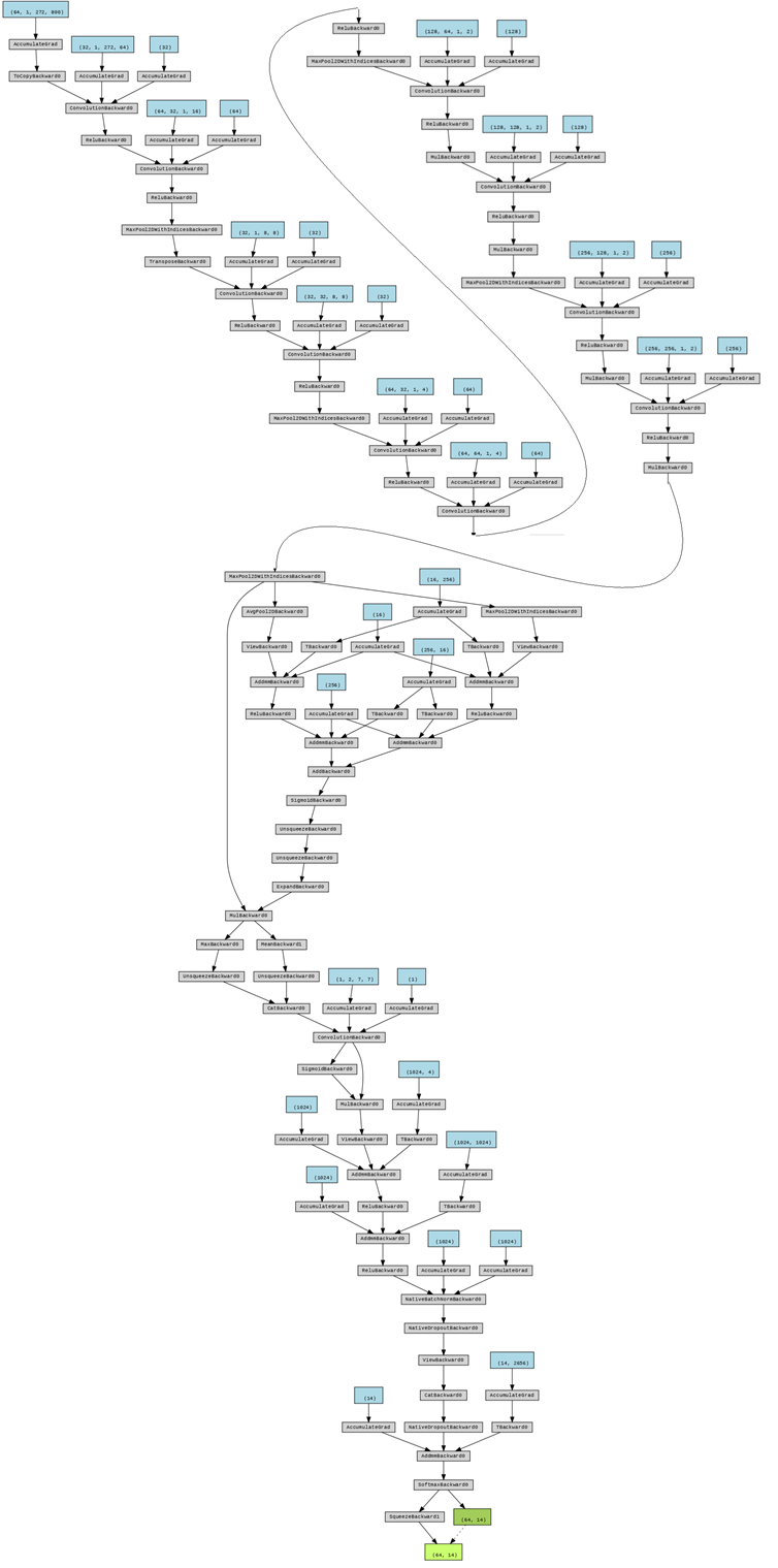
First save the model as .onnx file:

x = torch.randn(64, 1, 272, 800).requires_grad_(True).cuda() 
torch_out = rpsmnet(x)

# Export the model
torch.onnx.export(rpsmnet,               # model being run
                  x,                         # model input (or a tuple for multiple inputs)
                  "super_resolution.onnx",   # where to save the model (can be a file or file-like object)
                  export_params=True,        # store the trained parameter weights inside the model file
                  opset_version=10,          # the ONNX version to export the model to
                  do_constant_folding=True,  # whether to execute constant folding for optimization
                  input_names = ['input'],   # the model's input names
                  output_names = ['output'], # the model's output names
)

And I generate the flow chat of this model with Netron:

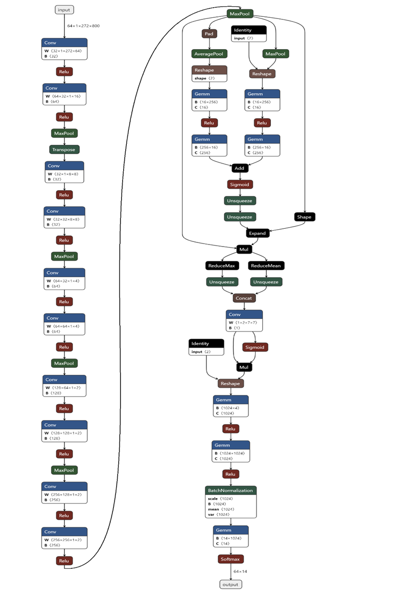
Detailed configuration of my model. Cov: convolution; Relu: rectified linear unit; MaxPool: max pooling; AveragePool: average pooling; Concat: concatenation; Identity: stands for relative power spectrum; Gemm: general matrix multiply

The steps data are processed is generated with following code:

import hiddenlayer as hl

transforms = [ hl.transforms.Prune('Constant') ] # Removes Constant nodes from graph.

graph = hl.build_graph(rpsmnet, torch.zeros(64,1,272,800).cuda())
graph.theme = hl.graph.THEMES['blue'].copy()
graph.save('ASRCnet_hiddenlayer', format='png')

from torchviz import make_dot
x = torch.randn(64, 1, 272, 800).requires_grad_(True).cuda() # 定义一个网络的输入值
y = rpsmnet(x)    # 获取网络的预测值
# y = y.cuda()
MyConvNetVis = make_dot(y)#, params=dict(list(rpsmnet.named_parameters()) + [('x', x)]))
MyConvNetVis.format = "png"
# 指定文件生成的文件夹
MyConvNetVis.directory = "data"
# 生成文件
MyConvNetVis.view()

July 15th

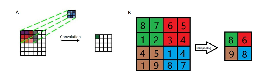
I want to visualize the pooling and convolution operations, so I use CAD to draw the illustrations:

As shown in figure A, a kernel filter is applied to the input data pixel: after summing up input values and filter, a result value is generated and passed to the next step. With all similar processes conducted step by step, a feature map is generated. Afterwards, the max pooling step (figure B) comes to decrease the dimensions of data in order to keep more neurons activated which is reported to reduce the overfitting as well